

3D structure and seasonal variation of temperature fronts in the shelf sea west of Guangdong
-
摘要: 基于2018–2019年现场高分辨率温度观测和1993–2021年的CMEMS再分析海表温度(SST)和风场数据,分析粤西陆架海温盐锋的三维结构、季节变化和影响机制。多年SST数据显示,海表温度锋冬季最强、出现概率和覆盖宽度最大,量值分别为0.049℃/km、75%和66 km。春季和夏季次之,而秋季则几乎完全消失。冬季锋面平均离岸50 km,夏季则向岸靠近为23.1 km。2018年春季、夏季和2019年夏季的现场观测进一步给出锋面在次表层的三维结构,结果显示春、夏季20 m等深线以浅处均有锋面存在,该锋面是沿岸高温海水与离岸低温海水辐聚而成,随着深度的增加锋面强度减小,覆盖范围向岸收缩。20 m以深水域锋面在次表层中强于表层,随深度增加而增强并向岸偏移。相关性和信息流分析发现,海表面风应力旋度和沿岸风是影响粤西陆架海表温度锋面的重要因素。该温度锋存在年际变化,PDO负位相时的La Niña年锋面强度出现极大值,而PDO正位相时的El Niño年则对应极小值。Abstract: Using reanalysis sea surface data and in-situ high-resolution observations in spring, summer 2018, and summer 2019, this study analyzes the 3D structure and seasonal variation of temperature fronts in the shelf sea west of Guangdong. The results show that the sea surface temperature (SST) fronts reach the strongest intensity up to 0.049°C/km in winter, with the largest occurrence probability of 75% and coverage of 66 km. The SST fronts weaken in spring and summer, and almost disappear in autumn. The average offshore distance of the front is 50 km in winter and 23.1 km in summer. The in-situ observations show a strong thermal front in coastal areas shallower than 20 m in both spring and summer. The front gets weaker and closer to the coast in deeper layers and is associated with warm coastal water and cold shelf water. In shelf areas deeper than 20 m, the fronts in the subsurface layer are stronger than in the surface layer and shift shoreward in deeper layers. The correlation coefficient and information flow between the surface wind and frontal parameters reveal that the surface wind stress curl and along-coast wind are the most important factors affecting the surface thermal front. These thermal fronts also have interannual variations, with maximum intensity in La Niña years with negative PDO and minimum intensity in El Niño years with positive PDO.
-
Key words:
- ocean front /
- seasonal variation /
- 3D structure /
- information flow /
- shelf west of Guangdong
-
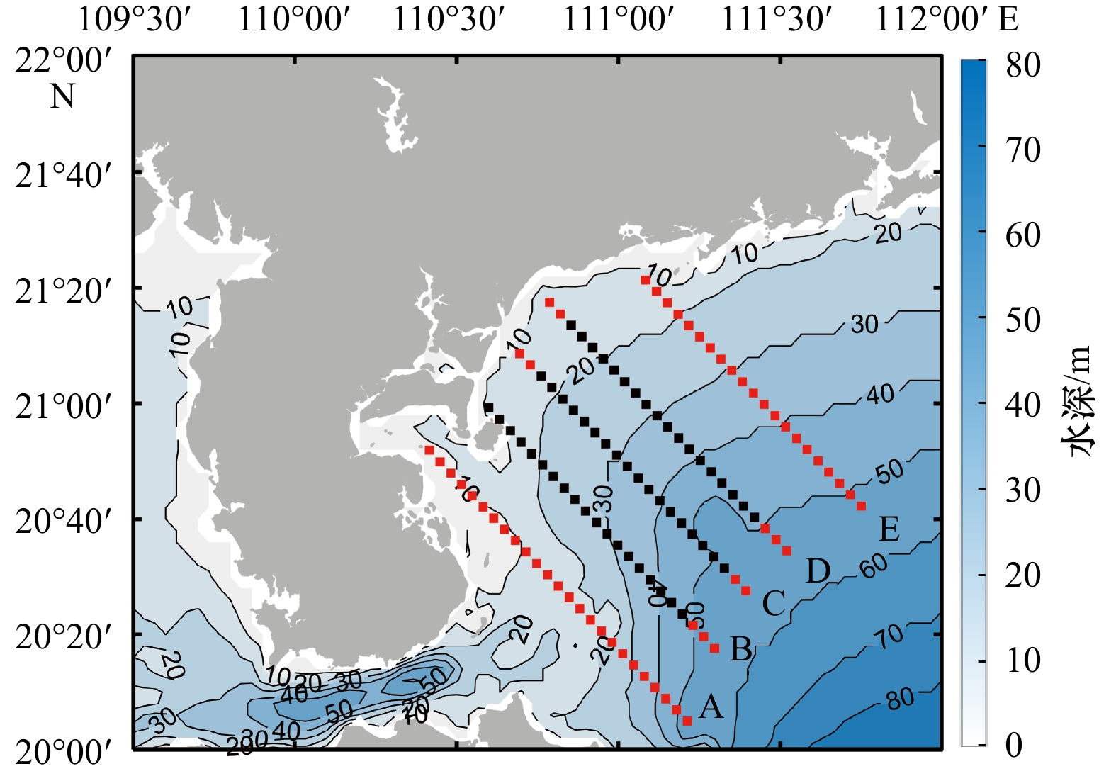
图 1 粤西陆架地形及2018和2019年观测站位分布
所有实心点为2018年观测站位,黑色实心点为2019年观测站位(红色点在2019年未观测)
Fig. 1 Bathymetry and observation stations on the shelf west of Guangdong in 2018 and 2019
All dots represent stations of which all are in 2018 and the black ones are in 2019 (the red dots were not observed in 2019)

图 2 海表面温度梯度的季节分布
a. 冬天;b. 春天;c. 夏天;d. 秋天。灰色等值线为水深,蓝色箭头为海面10 m风矢量
Fig. 2 Seasonal distribution of sea surface temperature gradient
a. Winter; b. spring; c. summer; d. autumn. Gray isolines represent the unter depth and blue arrows represent the wind vectors of 10 m on the sea surface

图 3 锋面出现概率的季节分布
a. 冬天;b. 春天;c. 夏天;d. 秋天。灰色等值线为水深,蓝色箭头为海面10 m风矢量,洋红色实线为锋面中心线
Fig. 3 Seasonal distribution of mean occurrence probabilities of the front at the sea surface
a. Winter; b. spring; c. summer; d. autumn. Gray isolines represent the unter depth and blue arrows represent the wind vectors of 10 m on the sea surface. The solid magenta line is the centerline of the front
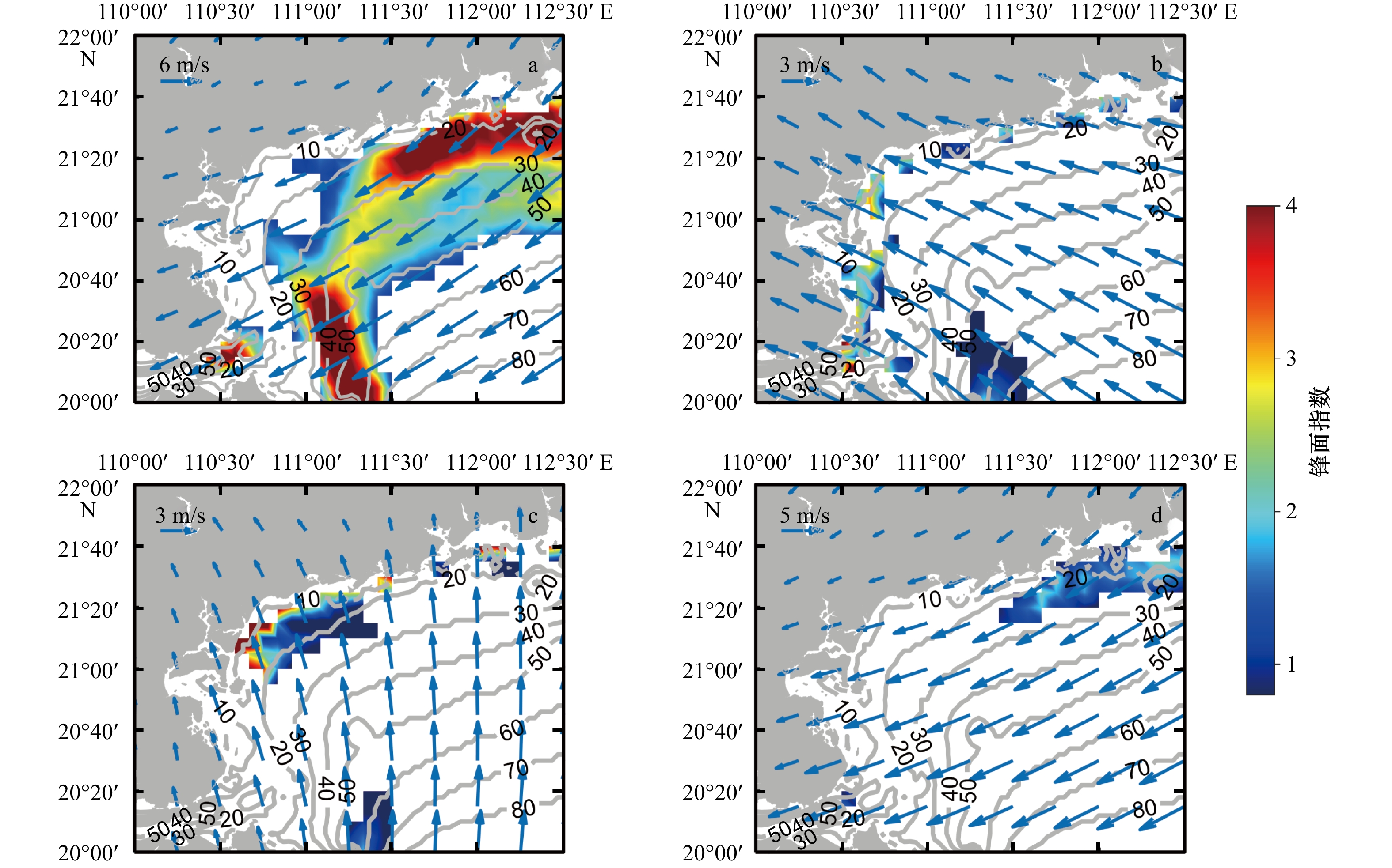
图 4 锋面指数I的季节分布
a. 冬天;b. 春天;c. 夏天;d. 秋天。灰色等值线为水深,蓝色箭头为海面10 m风矢量,洋红色实线为锋面中心线
Fig. 4 Seasonal distribution of front index I at the sea surface
a. Winter; b. spring; c. summer; d. autumn. Gray isolines represent the unter depth and blue arrows represent the surface wind vectors of 10 m on the sea surface. The solid magenta line is the centerline of the front
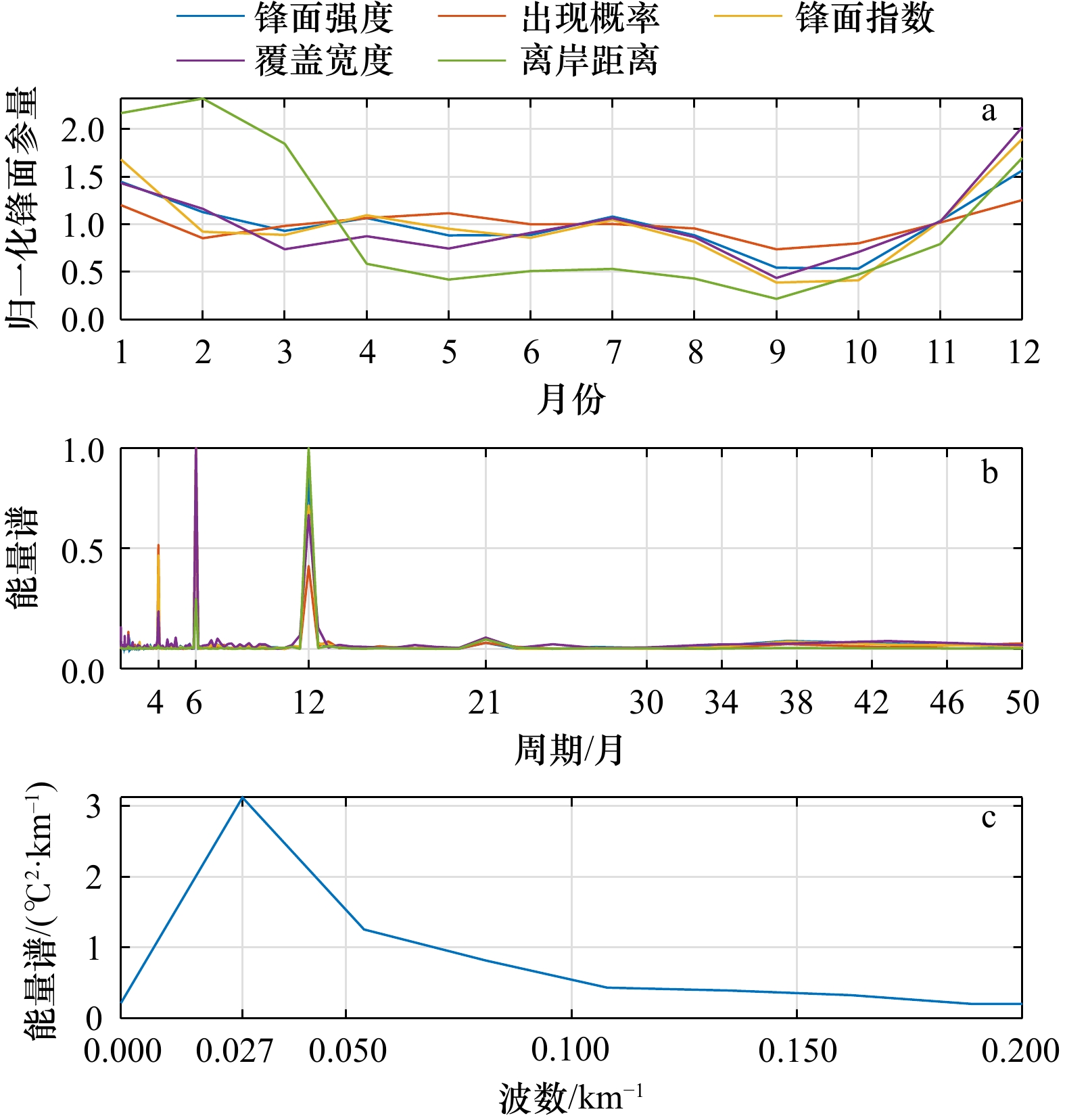
图 5 归一化后的5个锋面参量的月平均分布(a)、锋面参量的归一化FFT频率谱(b)和时间平均后锋面强度的FFT空间波数谱(c)
Fig. 5 Normalized monthly average distribution of the five frontal covariates (a), normalized FFT frequency spectrum of frontal covariates (b), omnidirectional time-average FFT spectra of frontal intensity (c)

图 6 现场观测航次期间平均CMEMS再分析SST和ECWMF再分析风场分布
a. 2018年春季;b. 2018年夏季;c. 2019年夏季。黑色实心点为站位,白色箭头为海面风矢量
Fig. 6 Sea surface temperature (SST) from CMEMS reanalysis data and sea surface wind field from ECWMF reanalysis data during the cruise observations
a. Spring 2018; b. summer 2018; c. summer 2019. The black dots represent stations, and the white arrows represent the surface wind vectors

图 7 2018年春季(a, d, g)、2018年夏季(b, e, h)和2019年夏季(c, f, i)观测温度水平分布
a–c为2 m,d–f为8 m,g–i为12 m。蓝色实线和灰色实线分别为海岸线和等深线
Fig. 7 Horizontal distribution of temperature in spring 2018 (a, d, g) , summer 2018 (b, e, h), and summer 2019 (c, f, i)
a–c at 2 m, d–f at 8 m, and g–i at 12 m. The blue and gray solid lines represent the coastline and isobaths, respectively

图 8 2018年春季(a, d, g)、2018年夏季(b, e, h)和2019年夏季(c, f, i)观测温度水平梯度分布
a–c为2 m,d–f 为8 m,g–i为12 m。蓝色实线和灰色实线分别为海岸线和等深线
Fig. 8 Horizontal distribution of temperature gradient in spring 2018 (a, d, g) , summer 2018 (b, e, h), and summer 2019 (c, f, i)
a–c at 2 m, d–f at 8 m, and g–i at 12 m. The blue and gray solid lines represent the coastline and isobaths, respectively
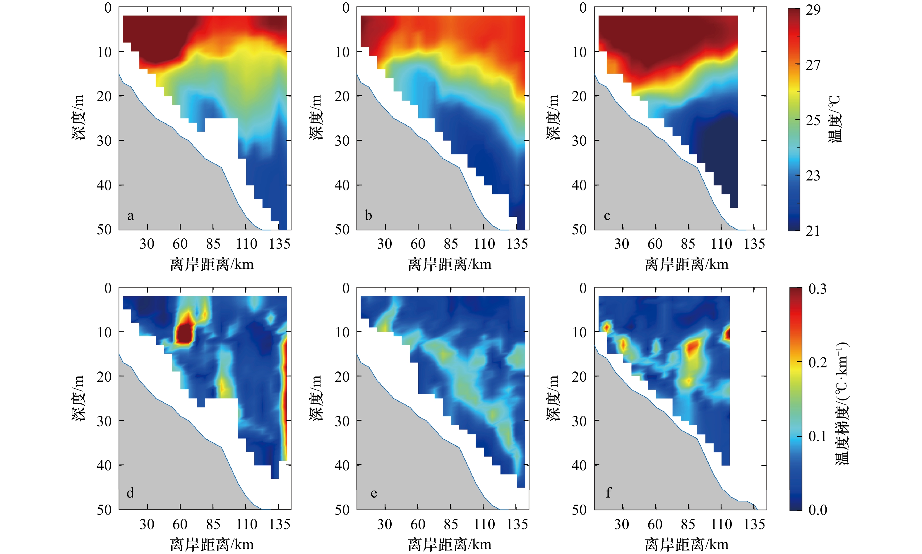
图 9 2018年春季(a, d)、夏季(b, e)和2019年夏季(c, f)C断面的温度(a–c),及温度梯度(d–f)垂直分布
Fig. 9 Vertical distribution of temperature (a–c) and gradient of temperature (d–f) at Section C in spring (a, d), summer 2018 (b, e), and summer 2019 (c, f)

图 10 1993–2021年月平均序列
虚线为原始月平均时间序列,实线为13个月低通滤波后的时间序列
Fig. 10 Time series of monthly-mean in 1993−2021
The dashed line is the original monthly-mean time series, and the solid line is the 13-month low-pass filtered time series
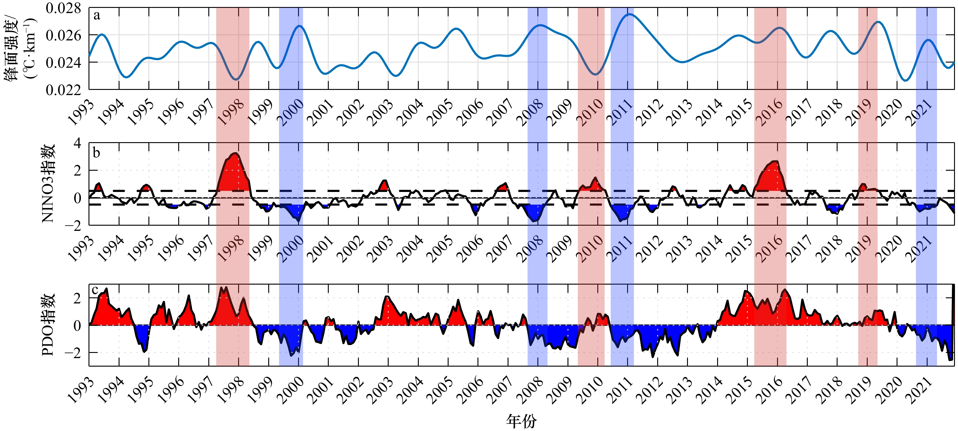
图 11 1993–2021年锋面强度(a)、NINO3指数(b)、 PDO指数(c)的时间序列
红色框为El Niño + PDO正位相,蓝色框为La Niña + PDO负位相
Fig. 11 Time series of frontal intensity (a), NINO3 index (b), and PDO index (c) in 1993–2021
Red boxes are El Niño + positive phase of PDO, and blue boxes are La Niña + negative phase of PDO

图 12 1993–2021年ENSO事件发生期间的SST分布
a. 1997–1998年El Niño;b. 2009–2010年El Niño;c. 2015–2016年El Niño;d. 2018–2019年El Niño;e. 1999–2000年La Niña;f. 2007–2008年La Niña;g. 2010–2011年La Niña;h. 2020–2021年La Niña。白色箭头为表面流速,黑色箭头为海上10 m风矢量,黑色实心点位置为锋面位置
Fig. 12 Distribution of SST during the 1993–2021 ENSO events
a. 1997–1998 El Niño; b. 2009–2010 El Niño; c. 2015–2016 El Niño; d. 2018–2019 El Niño; e. 1999–2000 La Niña; f. 2007–2008 La Niña; g. 2010–2011 La Niña; h. 2020–2021 La Niña. White arrows are surface currents, black arrows are offshore 10 m wind vector and the black solid dot position is the frontal areas
表 1 锋面参量与风参量的相关系数
Tab. 1 Correlation coefficient between frontal parameters and wind parameters
沿岸风应力
总体(冬,夏)向岸风应力
总体(冬,夏)风应力旋度
总体(冬,夏)风应力散度
总体(冬,夏)沿岸流
总体(冬,夏)锋面强度 0.45*(0.54, 0.50) 0.25*(0.55, 0.15) 0.47*(0.57, 0.3) 0.37*(0.13, 0.52) 0.42* (0.66, 0.56) 出现概率 0.42*(0.67, 0.51) 0.1(0.29, 0.1) 0.32*(0.65, 0.43) 0.32*(0.15, 0.46) 0.25* (0.59, 0.56) 覆盖宽度 0.52*(0.55, 0.58) 0.35*(0.45, 0.03) 0.51*(0.54, 0.47) 0.32*(0.51, 0.53) 0.13(0.62, 0.51) 离岸距离 0.38*(0.60, 0.53) –0.55*(–0.5, 0.24) 0.2*(0.36, 0.42) 0.2*(0.33, 0.1) 0.1(0.26, 0.22) 注:*表示相关系数通过95%的置信度检验,括号内分别为冬季(斜体)和夏季的相关系数。  下载: 导出CSV
表 2 锋面参量和风参量的信息流计算结果
Tab. 2 Information flow calculation results between frontal parameters and wind parameters
锋面强度 出现概率 覆盖宽度 离岸距离 沿岸风 向岸风 风应力旋度 锋面强度 – – – – 0.1 0.03 0.28 出现概率 – – – – 0.12 –0.002 0.14 覆盖宽度 – – – – 0.1 0.05 0.23 离岸距离 – – – – 0.22 0.29 0.09 沿岸风 –0.045 –0.017 –0.02 –0.08 – – – 向岸风 –0.03 –0.002 –0.05 0.008 – – – 风应力旋度 –0.14 –0.1 –0.12 –0.11 – – – 注:表中“–”为相同变量之间的结果,无意义。
下载: 导出CSV
-
[1] 鲍曼 M J, 埃萨阿斯 W E. 沿岸过程中的海洋锋[M]. 许建平, 刘仁清, 译. 北京: 海洋出版社, 1987.Bowman M J, Esaias W E. Oceanic Fronts in Coastal Processes[M]. Xu Jianping, Liu Renqing, trans. Beijing: China Ocean Press, 1987. [2] 冯士筰, 李凤岐, 李少菁. 海洋科学导论[M]. 北京: 高等教育出版社, 1999.Feng Shizuo, Li Fengqi, Li Shaojing. An Introduction to Marine Science[M]. Beijing: Higher Education Press, 1999. [3] Saldías G S, Hernández W, Lara C, et al. Seasonal variability of SST fronts in the Inner Sea of Chiloé and its adjacent coastal ocean, northern Patagonia[J]. Remote Sensing, 2021, 13(2): 181. doi: 10.3390/rs13020181 [4] Bost C A, Cotté C, Bailleul F, et al. The importance of oceanographic fronts to marine birds and mammals of the southern oceans[J]. Journal of Marine Systems, 2009, 78(3): 363−376. doi: 10.1016/j.jmarsys.2008.11.022 [5] Pollard R T, Regier L A. Vorticity and vertical circulation at an ocean front[J]. Journal of Physical Oceanography, 1992, 22(6): 609−625. doi: 10.1175/1520-0485(1992)022<0609:VAVCAA>2.0.CO;2 [6] Chelton D B, Esbensen S K, Schlax M G, et al. Observations of coupling between surface wind stress and sea surface temperature in the eastern Tropical Pacific[J]. Journal of Climate, 2001, 14(7): 1479−1498. doi: 10.1175/1520-0442(2001)014<1479:OOCBSW>2.0.CO;2 [7] Small R J, deSzoeke S P, Xie S P, et al. Air-sea interaction over ocean fronts and eddies[J]. Dynamics of Atmospheres and Oceans, 2008, 45(3/4): 274−319. [8] Ferrari R. A frontal challenge for climate models: an unusually detailed portrait of an ocean front off Japan could help improve climate predictions[J]. Science, 2011, 332(6027): 316−317. doi: 10.1126/science.1203632 [9] 宁修仁, 刘子琳, 蔡昱明. 我国海洋初级生产力研究二十年[J]. 东海海洋, 2000, 18(3): 13−20.Ning Xiuren, Liu Zilin, Cai Yuming. A review on primary production studies for China seas in the past 20 years[J]. Donghai Marine Science, 2000, 18(3): 13−20. [10] Li Q P, Zhou Weiwen, Chen Yinchao, et al. Phytoplankton response to a plume front in the northern South China Sea[J]. Biogeosciences, 2018, 15(8): 2551−2563. doi: 10.5194/bg-15-2551-2018 [11] Liu Zijia, Li Q P, Ge Zaiming, et al. Variability of plankton size distribution and controlling factors across a coastal frontal zone[J]. Progress in Oceanography, 2021, 197: 102665. doi: 10.1016/j.pocean.2021.102665 [12] Lü Ting, Liu Dongyan, Zhou Peng, et al. The coastal front modulates the timing and magnitude of spring phytoplankton bloom in the Yellow Sea[J]. Water Research, 2022, 220: 118669. doi: 10.1016/j.watres.2022.118669 [13] Hu Jianyu, Zhuang Wei, Zhu Jia, et al. Temperature, salinity and water mass in the South China Sea[M]//Hu Jianyu, Ho C R, Xie Lingling, et al. Regional Oceanography of the South China Sea. New Jersey: World Scientific, 2020: 43−75. [14] Xie Lingling, Zheng Quanan, Li Mingming, et al. Responses of the South China Sea to mesoscale disturbances from the Pacific[M]//Hu Jianyu, Ho C R, Xie Lingling, et al. Regional Oceanography of the South China Sea. New Jersey: World Scientific, 2020: 243−287. [15] Zhu Jia, Zheng Quanan, Hu Jianyu, et al. Classification and 3-D distribution of upper layer water masses in the northern South China Sea[J]. Acta Oceanologica Sinica, 2019, 38(4): 126−135. doi: 10.1007/s13131-019-1418-2 [16] 徐洪周, 许金电, 李立, 等. 2001年冬春转换期间南海东北部水文和环流特征[J]. 海洋学报, 2007, 29(5): 10−20.Xu Hongzhou, Xu Jindian, Li Li, et al. Hydrography and circulation characteristics about the northeast area of South China Sea during March 2001[J]. Haiyang Xuebao, 2007, 29(5): 10−20. [17] Yu Yi, Xing Xiaogang, Liu Hailong, et al. The variability of chlorophyll- a and its relationship with dynamic factors in the basin of the South China Sea[J]. Journal of Marine Systems, 2019, 200: 103230. doi: 10.1016/j.jmarsys.2019.103230 [18] 王磊, 王丽娅, 魏皓. 利用卫星遥感资料对南海北部陆架海洋表层温度锋的分析[J]. 中国海洋大学学报(自然科学版), 2004, 34(3): 351−357.Wang Lei, Wang Liya, Wei Hao. An analysis of the sea-surface thermal fronts in the northern shelf region of the South China Sea with satellite data[J]. Periodical of Ocean University of China, 2004, 34(3): 351−357. [19] Dong Jihai, Zhong Yisen. Submesoscale fronts observed by satellites over the northern South China Sea shelf[J]. Dynamics of Atmospheres and Oceans, 2020, 91: 101161. doi: 10.1016/j.dynatmoce.2020.101161 [20] 谢玲玲, 张书文, 赵辉. 琼东上升流研究概述[J]. 热带海洋学报, 2012, 31(4): 35−41.Xie Lingling, Zhang Shuwen, Zhao Hui. Overview of studies on Qiongdong upwelling[J]. Journal of Tropical Oceanography, 2012, 31(4): 35−41. [21] Wang Dongxiao, Liu Yun, Qi Yiquan, et al. Seasonal variability of thermal fronts in the northern South China Sea from satellite data[J]. Geophysical Research Letters, 2001, 28(20): 3963−3966. doi: 10.1029/2001GL013306 [22] 陈彪, 王静, 经志友, 等. 琼东和粤西海表温度锋的季节与年际变化特征分析[J]. 热带海洋学报, 2016, 35(5): 1−9.Chen Biao, Wang Jing, Jing Zhiyou, et al. Seasonal and interannual variation of thermal fronts off the east coast of Hainan Island and the west coast of Guangdong[J]. Journal of Tropical Oceanography, 2016, 35(5): 1−9. [23] Wang Y, Yu Y, Zhang Y, et al. Distribution and variability of sea surface temperature fronts in the South China Sea[J]. Estuarine, Coastal and Shelf Science, 2020, 240: 106793. doi: 10.1016/j.ecss.2020.106793 [24] Zhao Linhong, Yang Dingtian, Zhong Rong, et al. Interannual, seasonal, and monthly variability of sea surface temperature fronts in offshore China from 1982−2021[J]. Remote Sensing, 2022, 14(21): 5336. doi: 10.3390/rs14215336 [25] Jing Zhiyou, Qi Yiquan, Fox-Kemper B, et al. Seasonal thermal fronts on the northern South China Sea shelf: satellite measurements and three repeated field surveys[J]. Journal of Geophysical Research: Oceans, 2016, 121(3): 1914−1930. doi: 10.1002/2015JC011222 [26] Zhang Yan, Zeng Lili, Wang Qiang, et al. Seasonal variation in the three-dimensional structures of coastal thermal front off western Guangdong[J]. Acta Oceanologica Sinica, 2021, 40(7): 88−99. doi: 10.1007/s13131-021-1739-9 [27] Wang Guihua, Li Jiaxun, Wang Chunzai, et al. Interactions among the winter monsoon, ocean eddy and ocean thermal front in the South China Sea[J]. Journal of Geophysical Research: Oceans, 2012, 117(C8): C08002. [28] Yang Chaoyu, Ye Haibin. The features of the coastal fronts in the eastern Guangdong coastal waters during the downwelling-favorable wind period[J]. Scientific Reports, 2021, 11(1): 10238. doi: 10.1038/s41598-021-89649-8 [29] 经志友, 齐义泉, 华祖林. 南海北部陆架区夏季上升流数值研究[J]. 热带海洋学报, 2008, 27(3): 1−8.Jing Zhiyou, Qi Yiquan, Hua Zulin. Numerical study on summer upwelling over northern continental shelf of South China Sea[J]. Journal of Tropical Oceanography, 2008, 27(3): 1−8. [30] 许金电, 蔡尚湛, 宣莉莉, 等. 粤东至闽南沿岸海域夏季上升流的调查研究[J]. 热带海洋学报, 2014, 33(2): 1−9.Xu Jindian, Cai Shangzhan, Xuan Lili, et al. Observational study on summertime upwelling in coastal seas between eastern Guangdong and southern Fujian[J]. Journal of Tropical Oceanography, 2014, 33(2): 1−9. [31] Jing Zhiyou, Qi Yiquan, Du Yan. Upwelling in the continental shelf of northern South China Sea associated with 1997−1998 El Niño[J]. Journal of Geophysical Research: Oceans, 2011, 116(C2): C02033. [32] 谢玲玲, 宗晓龙, 伊小飞, 等. 琼东上升流的年际变化及长期变化趋势[J]. 海洋与湖沼, 2016, 47(1): 43−51.Xie Lingling, Zong Xiaolong, Yin Xiaofei, et al. The interannual variation and long-term trend of Qiongdong upwelling[J]. Oceanologia et Limnologia Sinica, 2016, 47(1): 43−51. [33] Xie Lingling, Pallàs-Sanz E, Zheng Quanan, et al. Diagnosis of 3D vertical circulation in the upwelling and frontal zones east of Hainan Island, China[J]. Journal of Physical Oceanography, 2017, 47(4): 755−774. doi: 10.1175/JPO-D-16-0192.1 [34] Geng Bingxu, Xiu Peng, Liu Na, et al. Biological response to the interaction of a mesoscale eddy and the river plume in the northern South China Sea[J]. Journal of Geophysical Research: Oceans, 2021, 126(9): e2021JC017244. doi: 10.1029/2021JC017244 [35] Chelton D B, Xie Shangping. Coupled ocean-atmosphere interaction at oceanic mesoscales[J]. Oceanography, 2010, 23(4): 52−69. doi: 10.5670/oceanog.2010.05 [36] Byrne D, Papritz L, Frenger I, et al. Atmospheric response to mesoscale sea surface temperature anomalies: assessment of mechanisms and coupling strength in a high-resolution coupled model over the South Atlantic[J]. Journal of the Atmospheric Sciences, 2015, 72(5): 1872−1890. doi: 10.1175/JAS-D-14-0195.1 [37] Oerder V, Colas F, Echevin V, et al. Mesoscale SST–wind stress coupling in the Peru–Chile current system: which mechanisms drive its seasonal variability?[J]. Climate Dynamics, 2016, 47(7): 2309−2330. [38] Li Jing, Shao Min. Response of Asian marine fishery to ENSO related SST for the period 1982−2016[J]. Oceanography & Fisheries Open access Journal, 2019, 9(3): 555763. [39] Wang Yuntao, Castelao R M. Variability in the coupling between sea surface temperature and wind stress in the global coastal ocean[J]. Continental Shelf Research, 2016, 125: 88−96. doi: 10.1016/j.csr.2016.07.011 [40] Liang X S. Unraveling the cause-effect relation between time series[J]. Physical Review E, 2014, 90(5): 052150. doi: 10.1103/PhysRevE.90.052150 [41] Liang X S. Normalizing the causality between time series[J]. Physical Review E, 2015, 92(2): 022126. [42] Lin Peigen, Cheng Peng, Gan Jianping, et al. Dynamics of wind-driven upwelling off the northeastern coast of Hainan Island[J]. Journal of Geophysical Research: Oceans, 2016, 121(2): 1160−1173. doi: 10.1002/2015JC011000 [43] 孙湘平. 中国近海区域海洋[M]. 北京: 海洋出版社, 2006: 109−110.Sun Xiangping. China Offshore Area[M]. Beijing: China Ocean Press, 2006: 109−110. [44] Wang Dongxiao, Hong Bo, Gan Jianping, et al. Numerical investigation on propulsion of the counter-wind current in the northern South China Sea in winter[J]. Deep-Sea Research Part I: Oceanographic Research Papers, 2010, 57(10): 1206−1221. doi: 10.1016/j.dsr.2010.06.007 [45] 谢玲玲, 曹瑞雪, 尚庆通. 粤西近岸环流研究进展[J]. 广东海洋大学学报, 2012, 32(4): 94−98.Xie Lingling, Cao Ruixue, Shang Qingtong. Progress of study on coastal circulation near the shore of western Guangdong[J]. Journal of Guangdong Ocean University, 2012, 32(4): 94−98. [46] Xue Huijie, Chai Fei, Pettigrew N, et al. Kuroshio intrusion and the circulation in the South China Sea[J]. Journal of Geophysical Research: Oceans, 2004, 109(C2): C02017. [47] Nan Feng, Xue Huijie, Chai Fei, et al. Identification of different types of Kuroshio intrusion into the South China Sea[J]. Ocean Dynamics, 2011, 61(9): 1291−1304. doi: 10.1007/s10236-011-0426-3 [48] Shu Yeqiang, Wang Qiang, Zu Tingting. Progress on shelf and slope circulation in the northern South China Sea[J]. Science China Earth Sciences, 2018, 61(5): 560−571. doi: 10.1007/s11430-017-9152-y [49] 朱凤芹, 谢玲玲, 成印河. 南海温度锋的分布特征及季节变化[J]. 海洋与湖沼, 2014, 45(4): 695−702.Zhu Fengqin, Xie Lingling, Cheng Yinhe. Distribution and seasonal variations of temperature front in the South China Sea[J]. Oceanologia et Limnologia Sinica, 2014, 45(4): 695−702. [50] 赵宝宏, 刘宇迪, 赵加华, 等. 南海海洋锋季节分布特征初探[C]//第28届中国气象学会年会——S17第三届研究生年会. 厦门: 中国气象学会, 2011.Zhao Baohong, Liu Yudi, Zhao Jiahua, et al. Seasonal distribution characteristics of ocean front in the South China Sea[C]//The 28th Annual Meeting of the China Meteorological Society. Xiamen: China Meteorological Society, 2011. [51] 郭艳君, 倪允琪. ENSO期间赤道太平洋对流活动异常对我国冬季风的影响[J]. 气象, 1998, 24(9): 3−7.Guo Yanjun, Ni Yunqi. Effects of the Tropical Pacific convective activities on China’s winter monsoon[J]. Meteorological Monthly, 1998, 24(9): 3−7. [52] Zhu Anbao, Xu Haiming, Deng Jiechun, et al. El Nino–Southern Oscillation (ENSO) effect on interannual variability in spring aerosols over East Asia[J]. Atmospheric Chemistry and Physics, 2021, 21(8): 5919−5933. doi: 10.5194/acp-21-5919-2021 -

计量
- 文章访问数: 1002
- HTML全文浏览量: 473
- PDF下载量: 84
- 被引次数: 0
