

Time-space continuous visualization of mesoscale vortices based on transfer function
-
摘要: 本文结合二维流线可视化技术和中尺度涡旋识别技术,提出了3种中尺度涡旋时空连续可视化的方法:基于OW参数的涡旋可视化方法、基于栅格模板的涡旋可视化方法和基于矢量模板的涡旋可视化方法,这3种方法分别基于Okubo-Weiss算法、Faghmous的算法和Liu的算法来进行涡旋识别,同时将流场可视化的结果填充到涡旋内部,以获得更好的可视化效果。在可视化过程中本文引入了传输函数来对涡旋中的流线颜色和透明度进行实时交互,能够在控制界面上通过设置Key值点的颜色和位置来控制速度、涡度和OW参数等信息的显示效果。本文在性能和显示效果方面比较了3种方法的优劣。从性能上来讲,性能由高到低依次为:基于OW参数的涡旋可视化方法、基于栅格模板的涡旋可视化方法和基于矢量模板的涡旋可视化方法。从显示效果上来讲,基于OW参数的涡旋可视化方法在三者中最差,效果中有较多的杂乱的短线,同时涡旋边界较小,局限于涡旋核心区;基于栅格模板的涡旋可视化方法较第一种方法的显示效果有所提升,杂乱的短线较少,涡旋相对完整,但由于数据分辨率不够高的原因,在放大多倍后涡旋边界呈现锯齿状;基于矢量模板的涡旋可视化方法显示效果最好,涡旋完整、饱满。同时,因为首先进行了涡旋边界的重构,将涡旋边界矢量化,涡旋边界更加平滑。相对于传统长时间序列的涡旋可视化的方法而言,这3种方法提供了一个美观、动态和更富信息性的可视化方法,同时由于传输函数的加入,其可以成为科研人员研究涡旋的一个实用的工具。Abstract: In this paper, three methods for continuous visualization of mesoscale eddies are proposed, which are based on the technique of 2D streamline visualization and technique of mesoscale eddies identification: the method of eddy visualization based on OW parameters, the method of eddy visualization based on grid template and the method of eddy visualization method based on vector template. These three methods are respectively based on Okubo-Weiss algorithm, Faghmous algorithm and Liu's algorithm for eddy recognition, and the visualization results of the flow field are filled into the eddy to obtain better visualization effect. In the process of visualization, we introduce the transfer function to conduct real-time interaction between the color and transparency of the streamline in the eddy, which can control the display effect of setting the velocity, vorticity, OW parameters and other information by setting the color and position of the Key point on the control interface. In addition, we also compared the advantages and disadvantages of the three methods in terms of performance and display effect. In terms of performance, the performance is from high to low: the method of eddy visualization based on OW parameters, the method of eddy visualization based on grid template and the method of eddy visualization method based on vector template. In terms of display effect, the method of eddy visualization based on OW parameters is the worst among the three, with more chaotic short lines and smaller eddy boundary, which is limited to the core region of the eddy. The method of eddy visualization based on grid template has better display effect than the first method, with fewer messy short lines and relatively complete eddy. However, due to the lack of high resolution of data, the eddy boundary appears jagged after being put up for more than one time. The method of eddy visualization method based on vector template has the best display effect. The eddy is complete and full. At the same time, since the eddy boundary is reconstructed and vectorized, the eddy boundary is smoother. Compared with the traditional method of continuous visualization of eddies with long time series, these three methods provide a beautiful, dynamic and more informative visualization method. At the same time, they can become a practical tool for researchers to study eddies due to the addition of transfer function.
-
Key words:
- eddy visualization /
- mesoscale eddy /
- transfer function
-

图 1 TIFF格式的MSLA-UV数据(2016年1月1日)
黄色区域为无效值区域,其他不同颜色表示流速差异
Fig. 1 MSLA-UV data in TIFF format(January 1, 2016)
The yellow area is the invalid value area, and other different colors indicate the flow rate difference
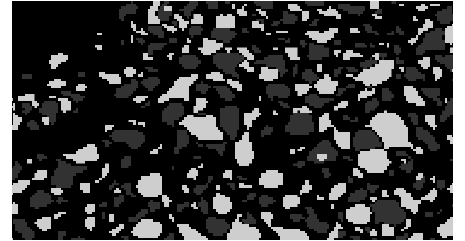
图 2 栅格模板数据(2016年1月1日)
黑色为无效值区域(大陆与北极冰雪覆盖地或非涡海域),浅灰色为冷涡,深灰色为暖涡
Fig. 2 Grid template data (January 1, 2016)
Black represents the invalid value area (continent and Arctic snow-covered areas or non-vortex sea areas), light gray represents cold vortex, and dark gray represents warm vortex
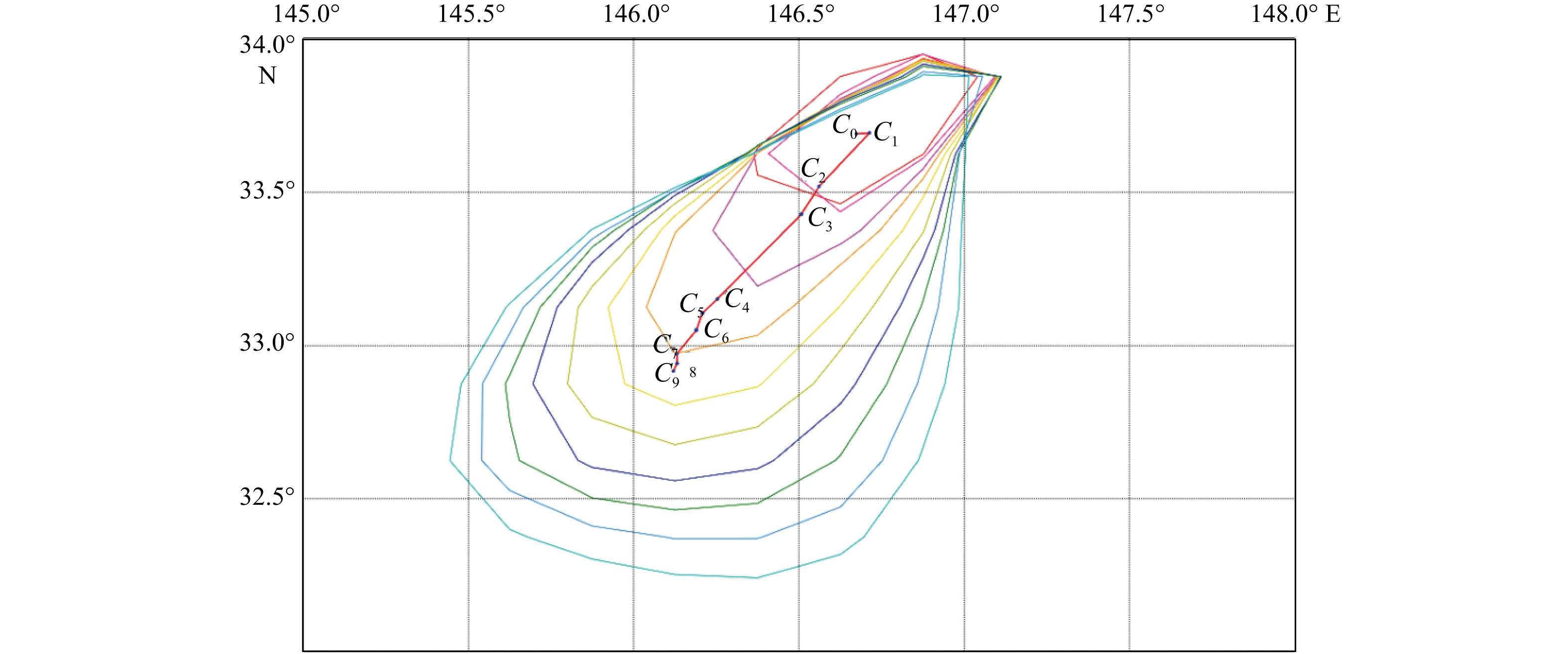
图 4 涡旋追踪结果示意图
红色折线是涡心所经过的路径,折线上的黑色圆点为涡心位置
Fig. 4 Schematic diagram of eddy tracking results
The red line is the path through the eddy center, and the black dots on the red line are the position of the eddy center

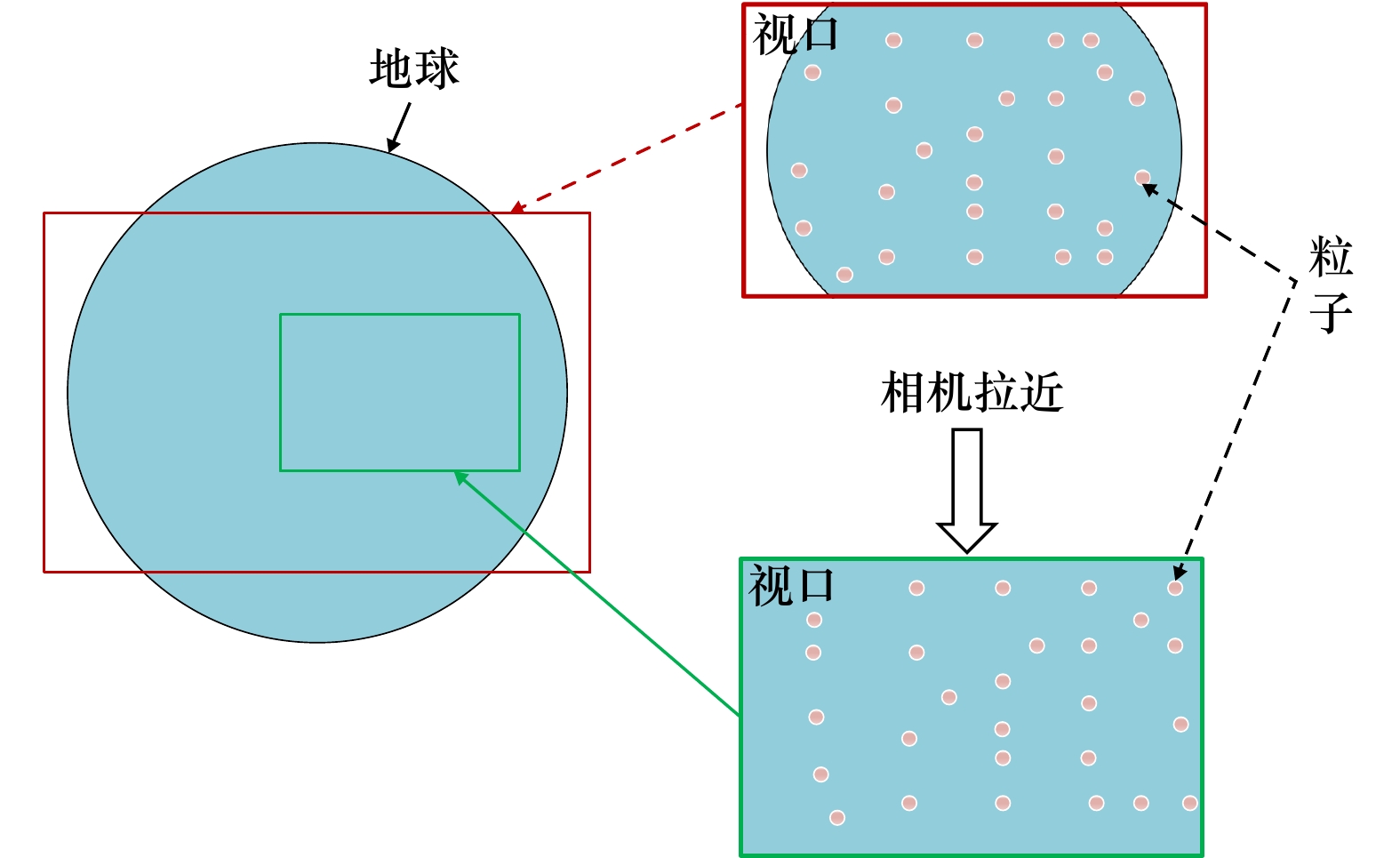
图 6 粒子密度随相机变化示意图(视口内播撒的粒子数目相同)
Fig. 6 Schematic diagram of particle density changing with the camera(the number of particles in the viewport are the same)
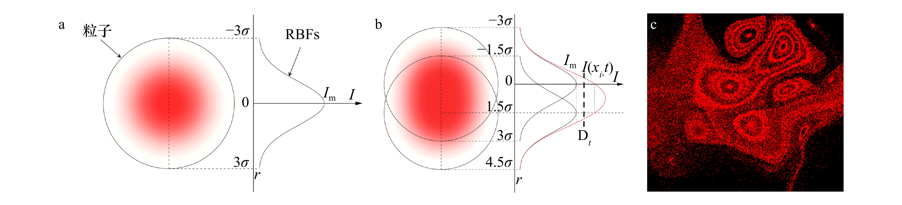
图 7 单个粒子的影响域(a),两个粒子的影响域叠加(b)和局部的概率密度图(c)
Fig. 7 The influence domain of a single particle (a), the superposition of the influence domain of two particles (b), and the local probability density diagram (c)
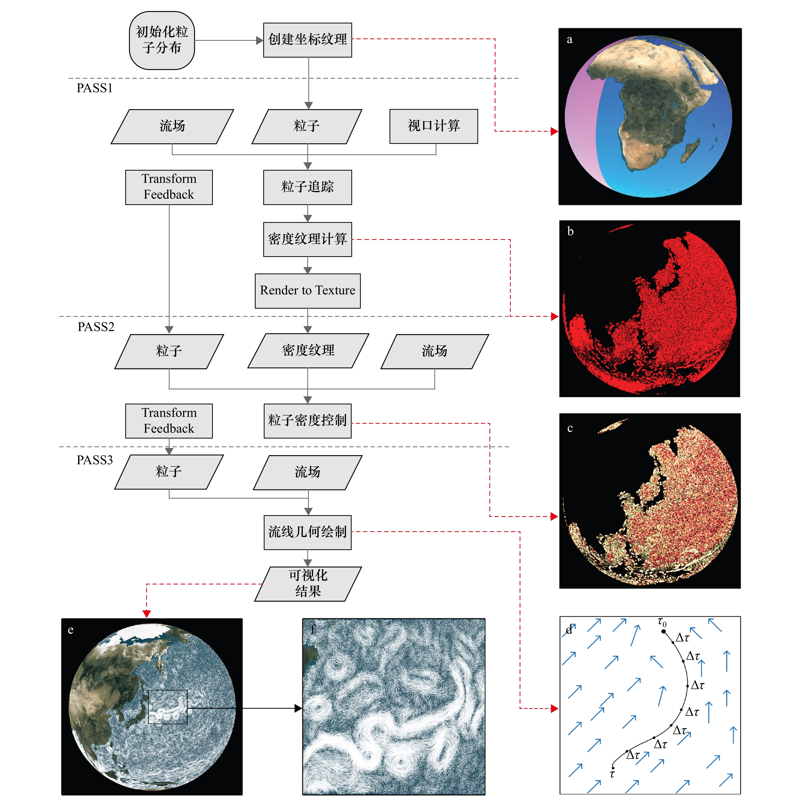
图 8 二维流线可视化流程图
a.坐标纹理;b.概率密度纹理;c.颜色表示年龄信息的密度纹理,粒子年龄为0时,颜色为白色,年龄在[0,1]时为黄色,年龄在[2,3]时颜色为红色;d.逐步积分生成流线,$ {\tau }_{0} $为起点,$ \tau $为终点;e.地球表面生成的流线;f.地球表面生成流线的局部放大图
Fig. 8 2D streamline visualization flowchart
a. coordinates texture; b. probability density texture; c. color represents the age information of density texture; when the particle’s age is 0, the color is white; when the age is [0,1], it is yellow; when the age is [2,3], it is red. d. step-by-step generation of streamlines, $ {\tau }_{0} $ and $ \tau $ are the beginning and end of integral time; e. streamlines on the earth’s surface; f. local magnification of streamlines on the earth’s surface
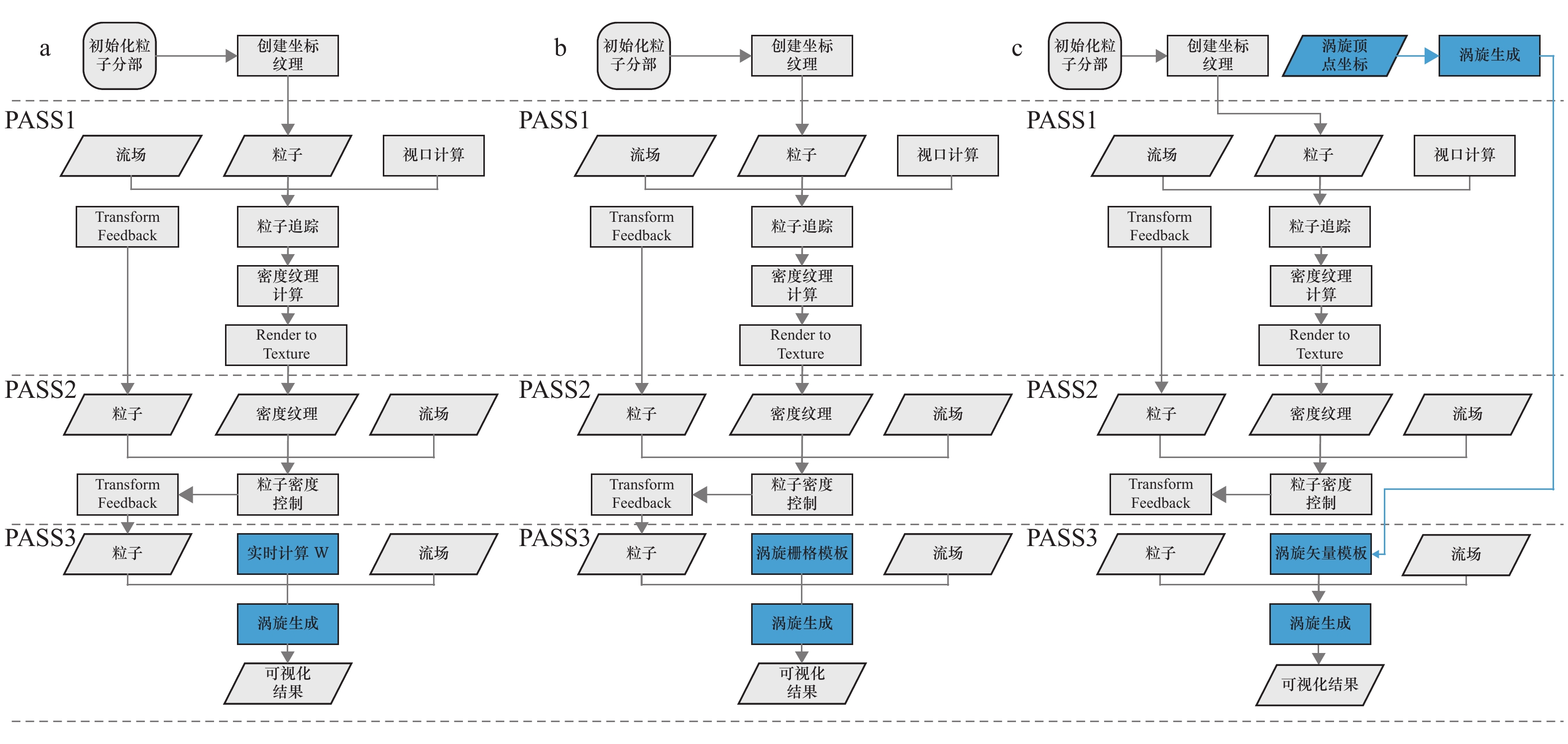
图 9 OW方法(a)、栅格方法(b)和矢量方法(c)的可视化流程图
与流线可视化主要区别在PASS3中的蓝色部分
Fig. 9 Visual flow charts of OW method (a), grid method (b) and vector method (c)
The main difference from streamline visualization is in the blue section of PASS3
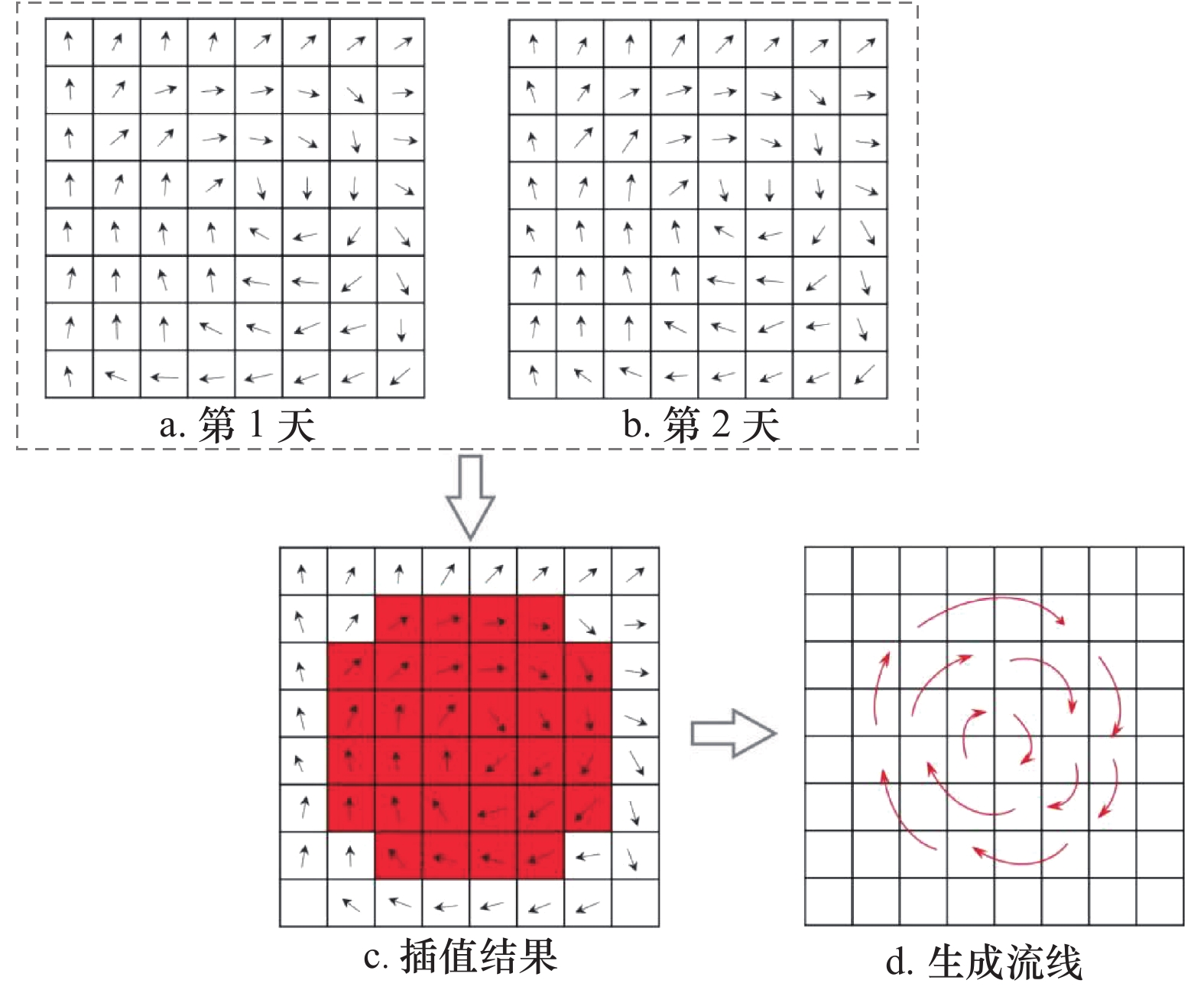
图 10 OW方法插值过程示意图
Fig. 10 A schematic diagram of the interpolation process in OW method
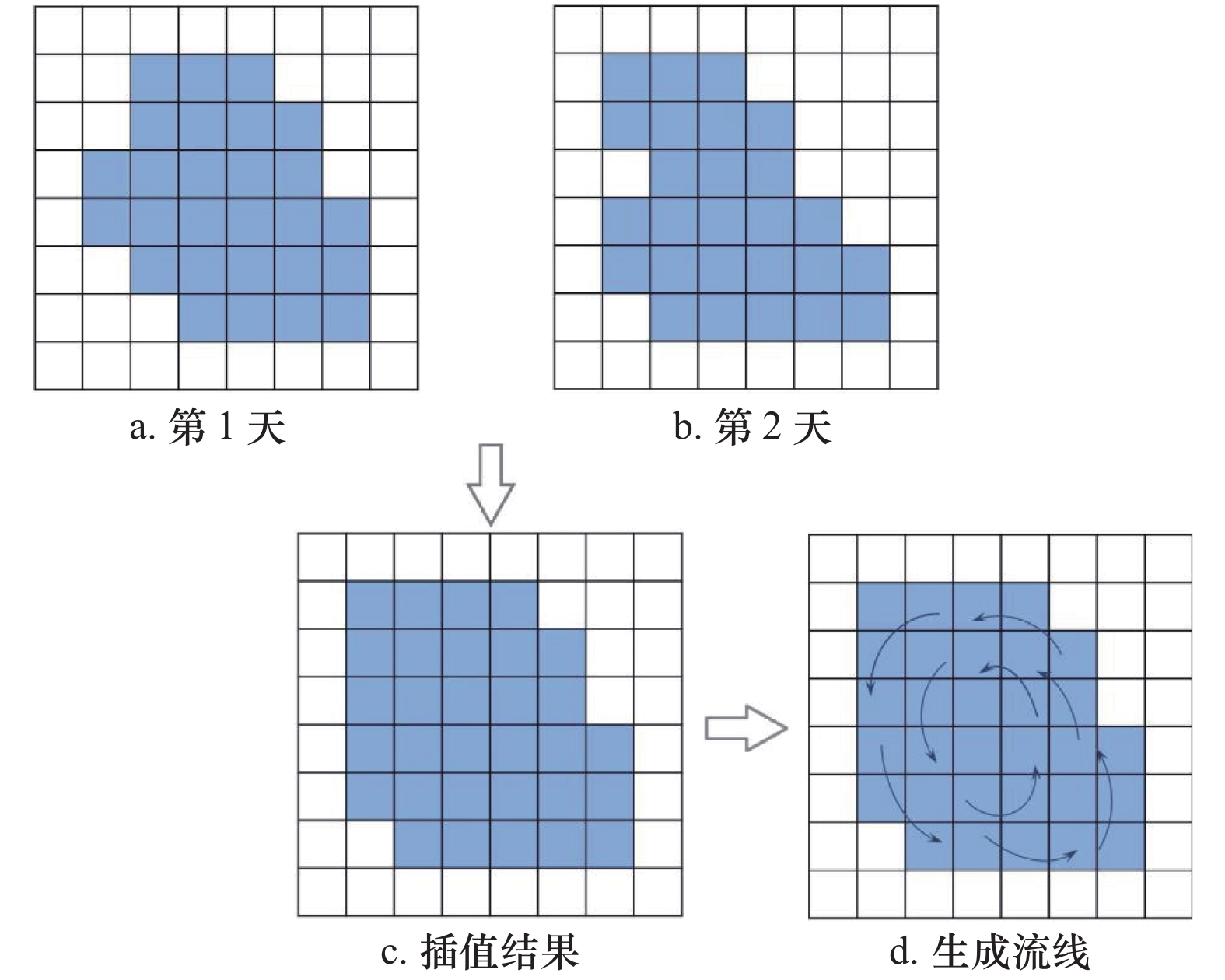
图 11 栅格方法插值过程示意图
Fig. 11 A schematic diagram of the interpolation process in grid method
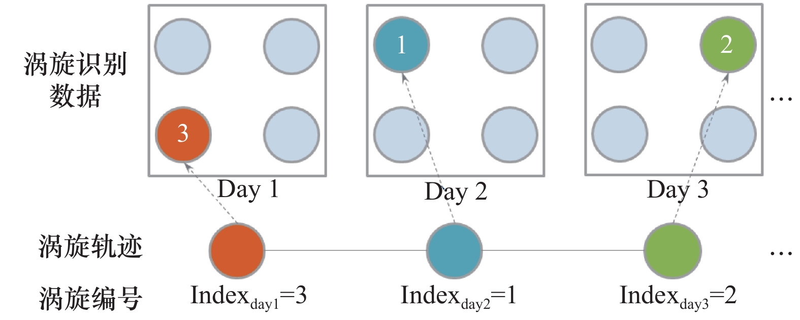
图 12 追踪数据与识别数据的关系示意图
Fig. 12 Schematic diagram of the relationship between tracking data and identifying data
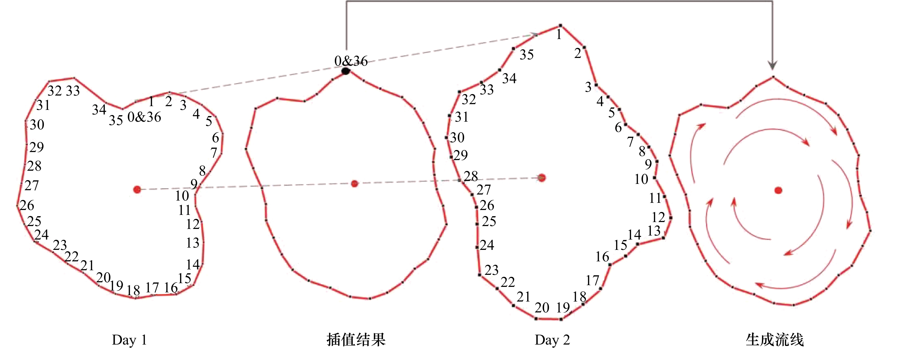
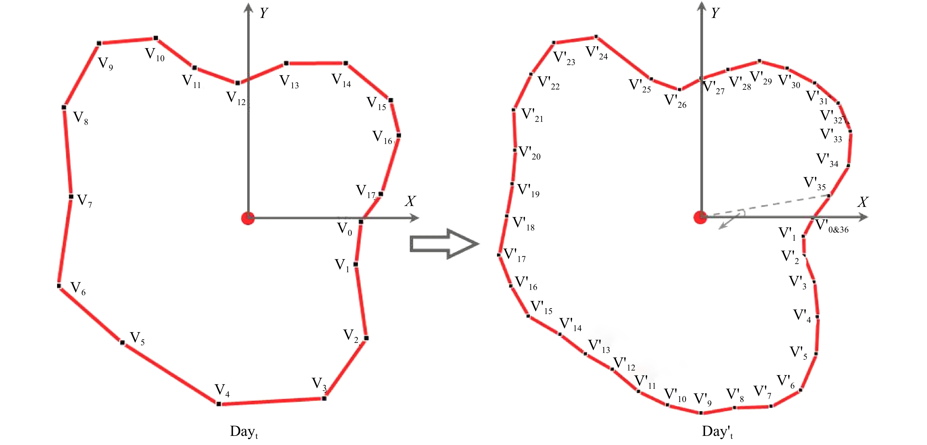
图 13 重构数据的顶点坐标插值示意图
Fig. 13 Interpolation diagram of vertex coordinates of reconstructed data

图 15 3种方法绘制的涡旋可视化结果(2016年1月1日)
第一、二、三行分别为OW方法、栅格方法、矢量方法绘制的结果,第一、二、三列的传输函数分别为W值、涡度和速度。传输函数中W参数和涡度的横坐标值都被放大了1010倍。涡度值的正号表示反气旋涡,负号表示气旋涡;W参数值大于0的部分被移除,将气旋涡的W参数的绝对值取代了W参数大于0的部分
Fig. 15 Visualization renderings of the three methods (January 1, 2016)
The first, second and third rows are drawn by OW method, grid method and vector method, respectively. The transmission functions of the first, second and third columns are W value, vorticity and velocity, respectively. The x-coordinate values of W parameter and vorticity in the transfer function are magnified 1010 times. The positive sign of vorticity value means anti-cyclonic and negative represents cyclonic. The part where the value of the W parameter is greater than zero is removed, and the part where the W parameter is greater than zero is replaced by the absolute value of the W parameter of cyclonic

图 16 OW方法(a)、栅格方法(b)、矢量方法(c)绘制的涡旋可视化效果局部放大图
Fig. 16 Local visualization renderings of OW method (a), grid method (b) and vector method (c)
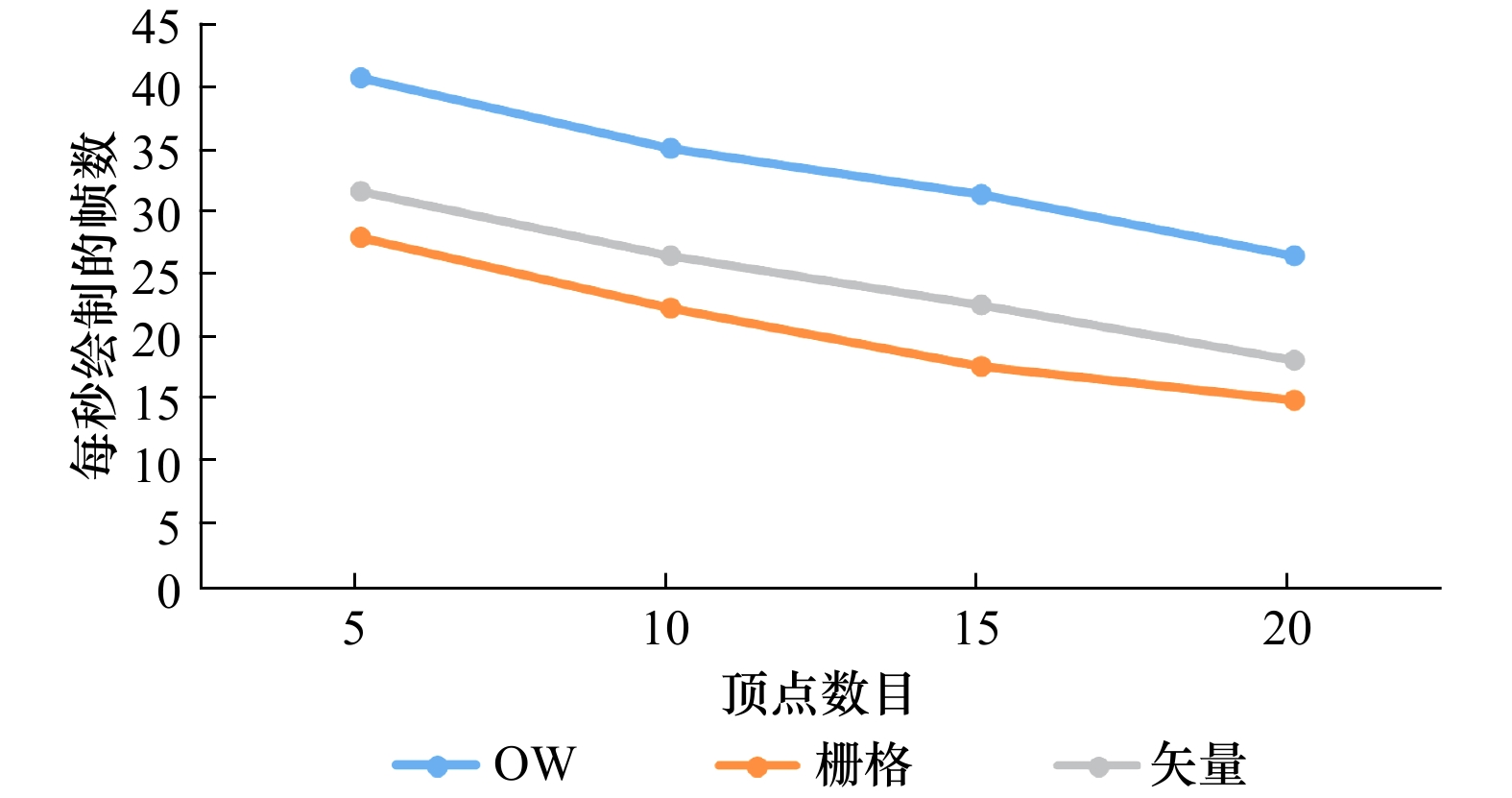
图 18 顶点数目对绘制效率的影响
Fig. 18 The effect of the number of vertices on rendering efficiency
-
[1] Williams S, Petersen M, Hecht M, et al. Interface exchange as an indicator for eddy heat transport[J]. Computer Graphics Forum, 2012, 31(3pt3): 1125−1134. doi: 10.1111/j.1467-8659.2012.03105.x [2] Faghmous J H, Le M, Uluyol M, et al. A parameter-free spatio-temporal pattern mining model to catalog global ocean dynamics[C]//2013 IEEE 13th International Conference on Data Mining. Dallas, TX, USA: IEEE, 2013. [3] Chaigneau A, Le Texier M, Eldin G, et al. Vertical structure of mesoscale eddies in the eastern South Pacific Ocean: A composite analysis from altimetry and Argo profiling floats[J]. Journal of Geophysical Research: Oceans, 2011, 116(C11): C11025. doi: 10.1029/2011JC007134 [4] Chelton D B, Gaube P, Schlax M G, et al. The influence of nonlinear mesoscale eddies on near-surface oceanic chlorophyll[J]. Science, 2011, 334(6054): 328−332. doi: 10.1126/science.1208897 [5] Chen Gengxin, Hou Yijun, Chu Xiaoqing. Mesoscale eddies in the South China Sea: Mean properties, spatiotemporal variability, and impact on thermohaline structure[J]. Journal of Geophysical Research: Oceans, 2011, 116(C6): C06018. [6] Dong Changming, Liu Yu, Lumpkin R, et al. A scheme to identify loops from trajectories of oceanic surface drifters: an application in the Kuroshio extension region[J]. Journal of Atmospheric and Oceanic Technology, 2011, 28(9): 1167−1176. doi: 10.1175/JTECH-D-10-05028.1 [7] 董昌明, 蒋星亮, 徐广珺, 等. 海洋涡旋自动探测几何方法、涡旋数据库及其应用[J]. 海洋科学进展, 2017, 35(4): 439−453. doi: 10.3969/j.issn.1671-6647.2017.04.001Dong Changming, Jiang Xingliang, Xu Guangjun, et al. Automated eddy detection using geometric approach, eddy datasets and their application[J]. Advances in Marine Science, 2017, 35(4): 439−453. doi: 10.3969/j.issn.1671-6647.2017.04.001 [8] Okubo A. Horizontal dispersion of floatable particles in the vicinity of velocity singularities such as convergences[J]. Deep Sea Research and Oceanographic Abstracts, 1970, 17(3): 445−454. doi: 10.1016/0011-7471(70)90059-8 [9] Weiss J. The dynamics of enstrophy transfer in two-dimensional hydrodynamics[J]. Physica D: Nonlinear Phenomena, 1991, 48(2/3): 273−294. [10] Sadarjoen I A, Post F H. Detection, quantification, and tracking of vortices using streamline geometry[J]. Computers & Graphics, 2000, 24(3): 333−341. [11] Nencioli F, Dong Changming, Dickey T, et al. A vector geometry-based eddy detection algorithm and its application to a high-resolution numerical model product and high-frequency radar surface velocities in the southern California bight[J]. Journal of Atmospheric and Oceanic Technology, 2010, 27(3): 564−579. doi: 10.1175/2009JTECHO725.1 [12] Liu Yingjie, Chen Ge, Sun Miao, et al. A parallel SLA-based algorithm for global Mesoscale eddy identification[J]. Journal of Atmospheric and Oceanic Technology, 2016, 33(12): 2743−2754. doi: 10.1175/JTECH-D-16-0033.1 [13] Faghmous J H, Frenger I, Yao Yuanshun, et al. A daily global mesoscale ocean eddy dataset from satellite altimetry[J]. Scientific Data, 2015, 2: 150028. doi: 10.1038/sdata.2015.28 [14] Jobard B, Lefer W. Creating evenly-spaced streamlines of arbitrary density[M]//Lefer W, Grave M. Visualization in Scientific Computing’97. Vienna: Springer, 1997: 43−55. [15] Jobard B, Lefer W. Unsteady flow visualization by animating evenly-spaced streamlines[J]. Computer Graphics Forum, 2000, 19(3): 31−39. doi: 10.1111/1467-8659.00395 [16] Liu Zhanping, Moorhead R, Groner J. An advanced evenly-spaced streamline placement algorithm[J]. IEEE Transactions on Visualization and Computer Graphics, 2006, 12(5): 965−972. doi: 10.1109/TVCG.2006.116 [17] Liu Zhanping, Moorhead II R J. Interactive view-driven evenly spaced streamline placement[C]//Proceedings of SPIE 6809, Visualization and Data Analysis 2008. San Jose, California, United States: SPIE, 2008: 68090A. [18] Weiskopf D, Schramm F, Erlebacher G, et al. Particle and texture based spatiotemporal visualization of time-dependent vector fields[C]//VIS 05. IEEE Visualization, 2005. Minneapolis, MN, USA: IEEE, 2005: 639−646. [19] Pighin F, Cohen J M, Shah M. Modeling and editing flows using advected radial basis functions[C]//Proceedings of the 2004 ACM SIGGRAPH/Eurographics Symposium on Computer Animation. Goslar, Germany: Eurographics Association, 2004. [20] 何珏, 田丰林, 张昉, 等. 基于实时几何流线生成的二维海流数据交互可视化方法[J]. 海洋技术学报, 2015, 34(3): 91−96.He Jue, Tian Fenglin, Zhang Fang, et al. Study on the interactive visualization method of 2D ocean current data based on real-time geometric streamline generation[J]. Journal of Ocean Technology, 2015, 34(3): 91−96. [21] Tian Fenglin, Cheng Lingqi, Chen Ge. Transfer function-based 2D/3D interactive spatiotemporal visualizations of mesoscale eddies[J]. International Journal of Digital Earth, 2018, 13(5): 546−566. [22] Kindlmann G, Durkin J W. Semi-automatic generation of transfer functions for direct volume rendering[C]//IEEE Symposium on Volume Visualization (Cat. No. 989EX300). Research Triangle Park, NC, USA: IEEE, 1998. [23] Sereda P, Bartroli A V, Serlie I W O, et al. Visualization of boundaries in volumetric data sets using LH histograms[J]. IEEE Transactions on Visualization and Computer Graphics, 2006, 12(2): 208−218. doi: 10.1109/TVCG.2006.39 [24] Helgeland A, Andreassen O. Visualization of vector fields using seed LIC and volume rendering[J]. IEEE Transactions on Visualization and Computer Graphics, 2004, 10(6): 673−682. doi: 10.1109/TVCG.2004.49 [25] Copernicus Programme. Global ocean gridded l4 sea surface heights and derived variables reprocessed (1993-ongoing)[R/OL]. (2016-01-01) [2019-05-30]. http://marine.copernicus.eu/services-portfolio/access-to-products/?option=com_csw&view=details&product_id=SEALEVEL_GLO_PHY_L4_REP_OBSERVATIONS_008_047. [26] Copernicus Programme. Global ocean gridded l4 sea surface heights and derived variables reprocessed (copernicus climate service)[R/OL]. (2016-01-01) [2019-05-30]. http://marine.copernicus.eu/services-portfolio/access-to-products/?option=com_csw&view=details&product_id=SEALEVEL_GLO_PHY_CLIMATE_L4_REP_OBSERVATIONS_008_057. [27] Sun Miao, Tian Fenglin, Liu Yingjie, et al. An improved automatic algorithm for global eddy tracking using satellite altimeter data[J]. Remote Sensing, 2017, 9(3): 206. doi: 10.3390/rs9030206 [28] 陈为, 沈则潜, 陶煜波. 数据可视化[M]. 北京: 电子工业出版社, 2013: 268−270.Chen Wei, Shen Zeqian, Tao Yubo. Data Visualization[M]. Beijing: Electronic Industry Press, 2013: 268−270. [29] Hansen C D, Johnson C R. Visualization Handbook[M]. Cambridge: Academic Press, 2011. [30] Ken Perlin. Improving noise[C]//Proceedings of the 29th Annual Conference on Computer Graphics and Interactive Techniques (SIGGRAPH'02). New York, NY, USA: Association for Computing Machinery, 2002: 681-682. [31] Williams S, Hecht M, Petersen M, et al. Visualization and analysis of eddies in a global ocean simulation[J]. Computer Graphics Forum, 2011, 30(3): 991−1000. doi: 10.1111/j.1467-8659.2011.01948.x [32] Chen Changheng, Kamenkovich I, Berloff P. Eddy trains and striations in quasigeostrophic simulations and the ocean[J]. Journal of Physical Oceanography, 2016, 46(9): 2807−2825. doi: 10.1175/JPO-D-16-0066.1 [33] 杨光. 西北太平洋中尺度涡旋研究[D]. 青岛: 中国科学院海洋研究所, 2013.Yang Guang. A study on the mesoscale eddies in the northwestern Pacific Ocean[D]. Qingdao: The Institute of Oceanology, Chinese Academy of Science, 2013. [34] Nieto K, McClatchie S, Weber E D, et al. Effect of mesoscale eddies and streamers on sardine spawning habitat and recruitment success off southern and central California[J]. Journal of Geophysical Research: Oceans, 2014, 119(9): 6330−6339. doi: 10.1002/2014JC010251 [35] 崔凤娟. 南海中尺度涡的识别及统计特征分析[D]. 青岛: 中国海洋大学, 2015.Cui Fengjuan. Mesoscale eddies in the South China Sea: identification and statistical characteristics analysis[D]. Qingdao: Ocean University of China, 2015. [36] Souza J M A C, De Boyer Montégut C, Le Traon P Y. Comparison between three implementations of automatic identification algorithms for the quantification and characterization of mesoscale eddies in the South Atlantic Ocean[J]. Ocean Science Discussions, 2011, 8(2): 483−531. doi: 10.5194/osd-8-483-2011 [37] Shivamoggi B K, Van Heijst G J F, Kamp L P J. The Okubo-Weiss criteria in two-dimensional hydrodynamic and magnetohydrodynamic flows[J]. Physics, 2015, arXiv: 110.6190. -

 下载:
下载:


 点击查看大图
计量
- 文章访问数: 159
- HTML全文浏览量: 17
- PDF下载量: 18
- 被引次数: 0
