

Ocean available gravitational potential energy calculated through CMIP5 model outputs and Argo observations
-
摘要: 有效重力势能作为重力势能中活跃的部分,能够参与海洋能量循环。本文计算和评估了CMIP5中9个模式的全球大洋2 000 m以上积分的有效重力势能和200~500 m深度范围内的中尺度有效重力势能,并与由BOA_Argo观测数据计算的结果进行比较。分析表明,就全球大洋2 000 m以上积分的有效重力势能而言,多数模式的计算结果均大于由Argo观测数据计算的结果。通过比较有效重力势能的空间分布特征,发现在强动力活跃区(特别是黑潮、湾流、南极绕极流区),模式与观测相差较大,其差别主要来源于观测与模式中扰动密度的差异。此外,在黑潮和南大洋区域,涡动能和有效重力势能具有较高的时间相关性,而在北大西洋湾流区域,两者的相关性较低;功率谱分析显示中尺度有效重力势能与涡动能都存在显著的半年和年变化周期。Abstract: As the active part of gravitational potential energy (GPE), available gravitational potential energy (AGPE) can participate in ocean energy cycle. In this paper, we calculated the AGPE in the upper 2 000 m in the global ocean and the mesoscale AGPE within the depth range of 200−500 m from the outputs of 9 CMIP5 models. The results are compared with those calculated from BOA_Argo observational data. The results show that the basin scale AGPE calculated from model outputs are mostly larger than those obtained by Argo observations. In the areas with strong dynamic activities (especially the Kuroshio, gulf stream, the Antarctic Circumpolar Current), the AGPE calculated from model outputs show obvious difference from those obtained via the Argo observation, and the difference mainly comes from the density perturbation. The eddy kinetic energy (EKE) and the mesoscale AGPE have a remarkable temporal correlation in the Kuroshio and the Southern Ocean regions, but their correlation coefficient is low in the gulf stream region of North Atlantic. The power spectrum analysis shows that both the mesoscale AGPE and EKE have significant semi-annual and annual variablilities.
-
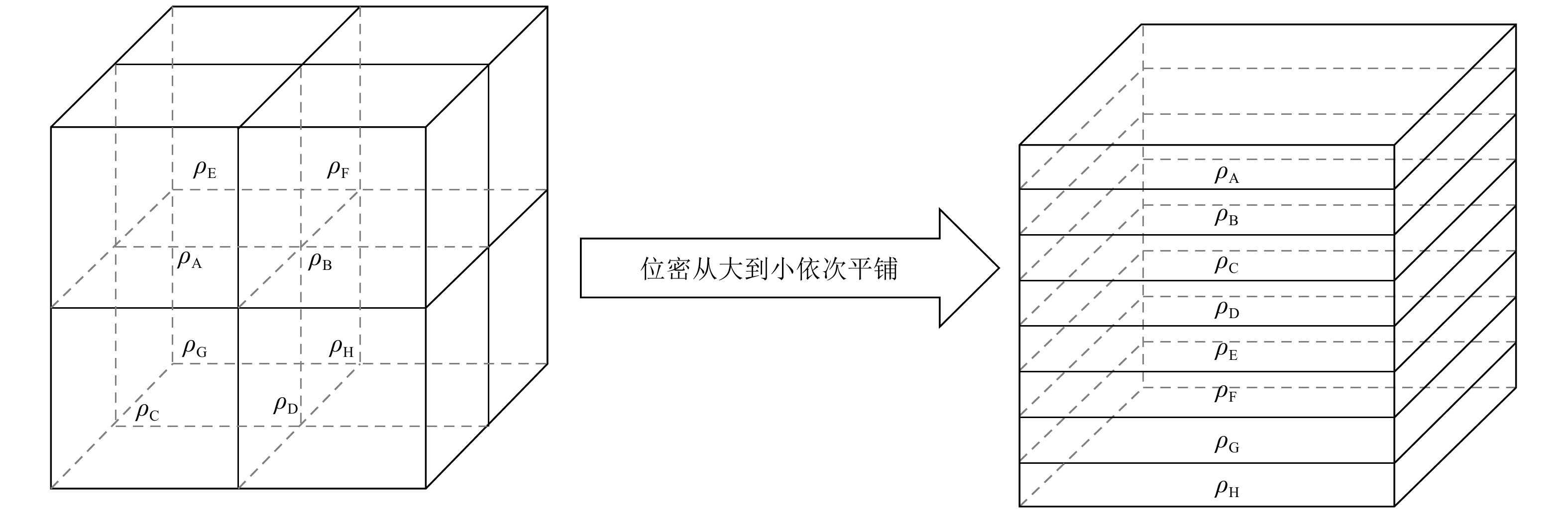
图 1 “迭代法”中计算三维海水参考势能图示
Fig. 1 A brief description of three dimensional seawater iteration method for calculating reference gravity potential energy

图 2 各模式计算的重力势能(GPE)、参考重力势能(RGPE)、有效重力势能(AGPE)与Argo观测结果的相对误差
Fig. 2 The relative bias of GPE, RGPE, AGPE between the model outputs and the Argo observations

图 3 Argo观测与各模式计算的重力势能(GPE)、参考重力势能(RGPE)、有效重力势能(AGPE)时间变化序列
Fig. 3 Time variations of GPE, RGPE and AGPE calculated from Argo observations and model outputs
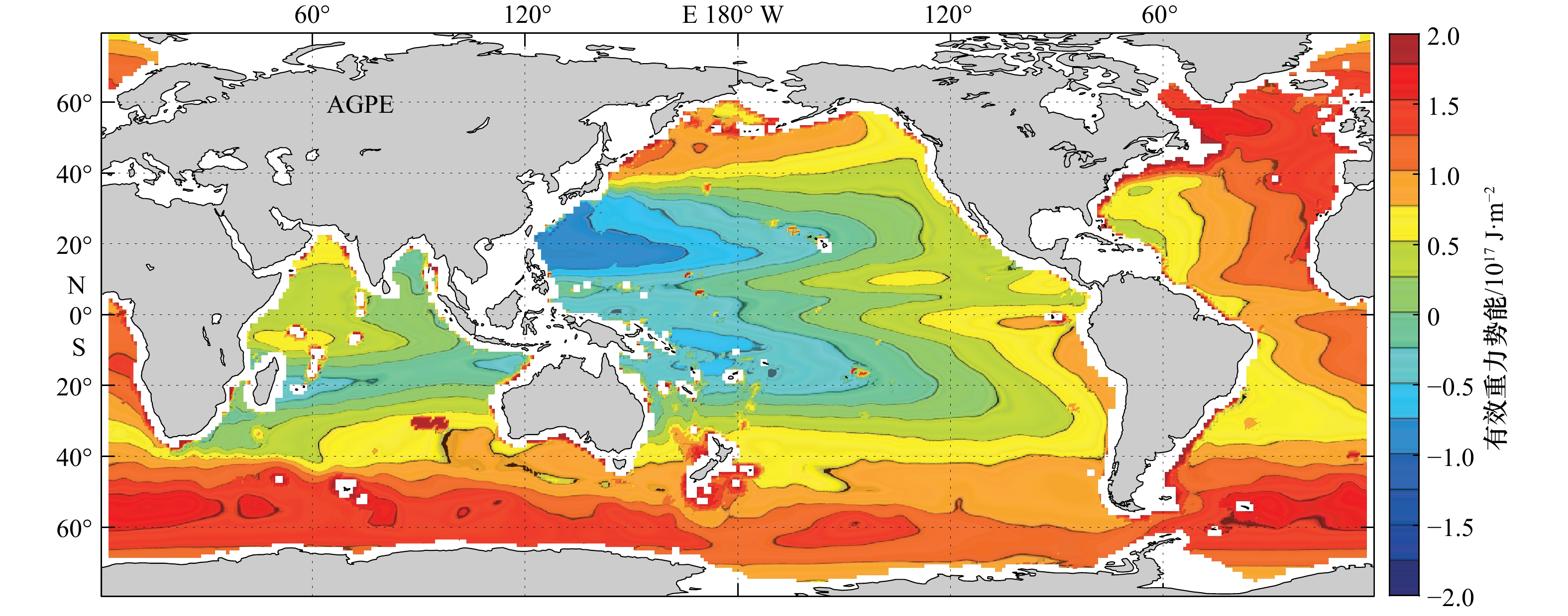
图 4 由Argo观测计算的海盆尺度有效重力势能(AGPE)空间分布
Fig. 4 Spatial distribution of AGPE at basin scale calculated from Argo observations
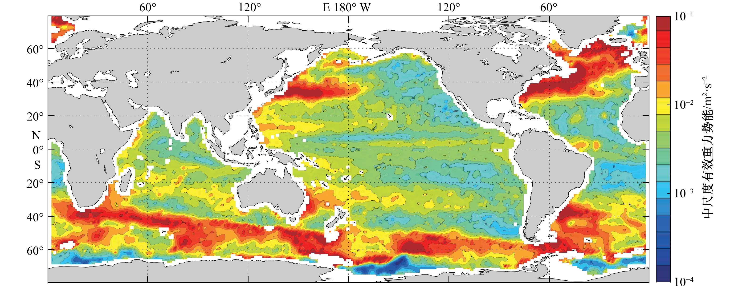
图 5 由Argo观测计算的200~500 m深度平均的中尺度有效重力势能(EAGPE)空间分布
Fig. 5 Spatial distribution of depth-averaged EAGPE between 200 m and 500 m calculated from Argo observations
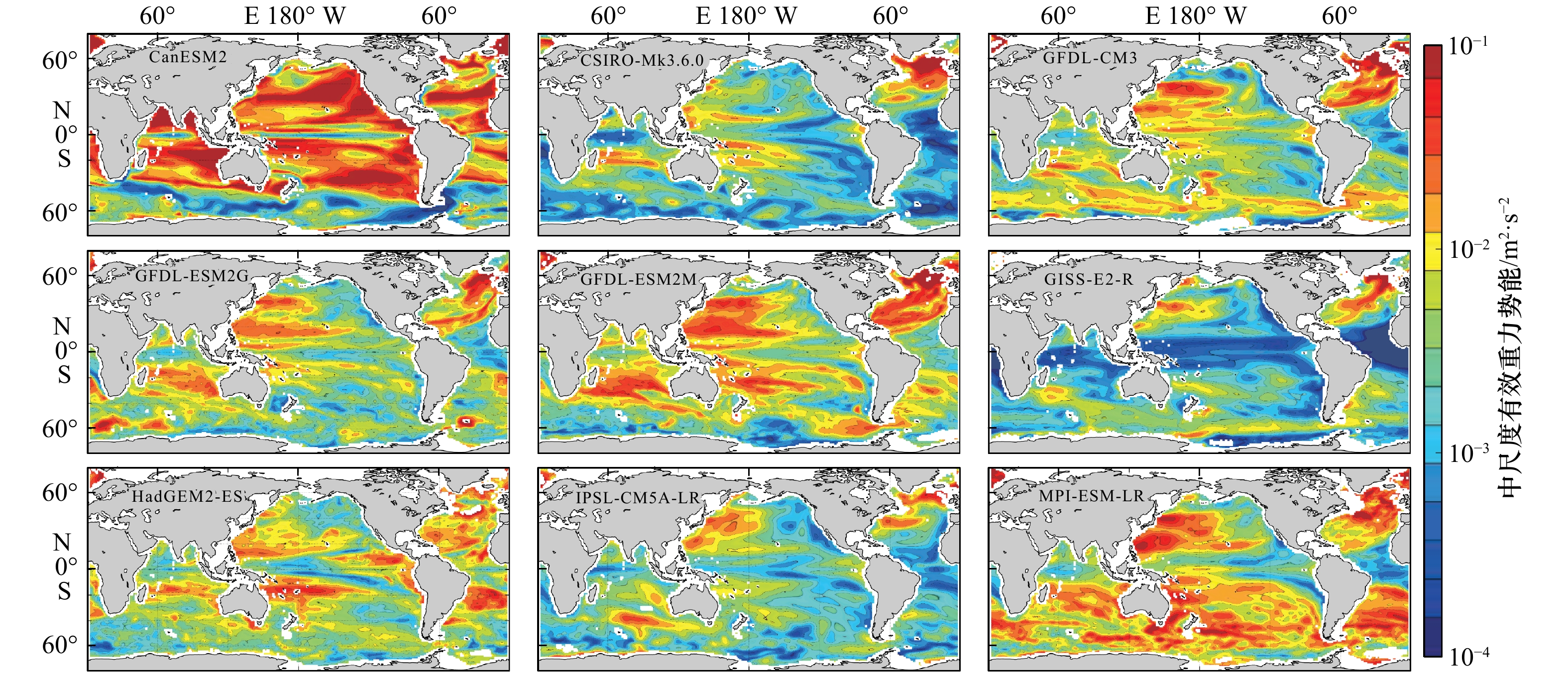
图 6 由模式计算的200~500 m深度平均的中尺度有效重力势能(EAGPE)空间分布
Fig. 6 Spatial distribution of depth-averaged EAGPE between 200 m and 500 m calculated from model outputs

图 7 各模式扰动密度平方项的空间分布
Fig. 7 Spatial distribution of the square of density perturbation in each model
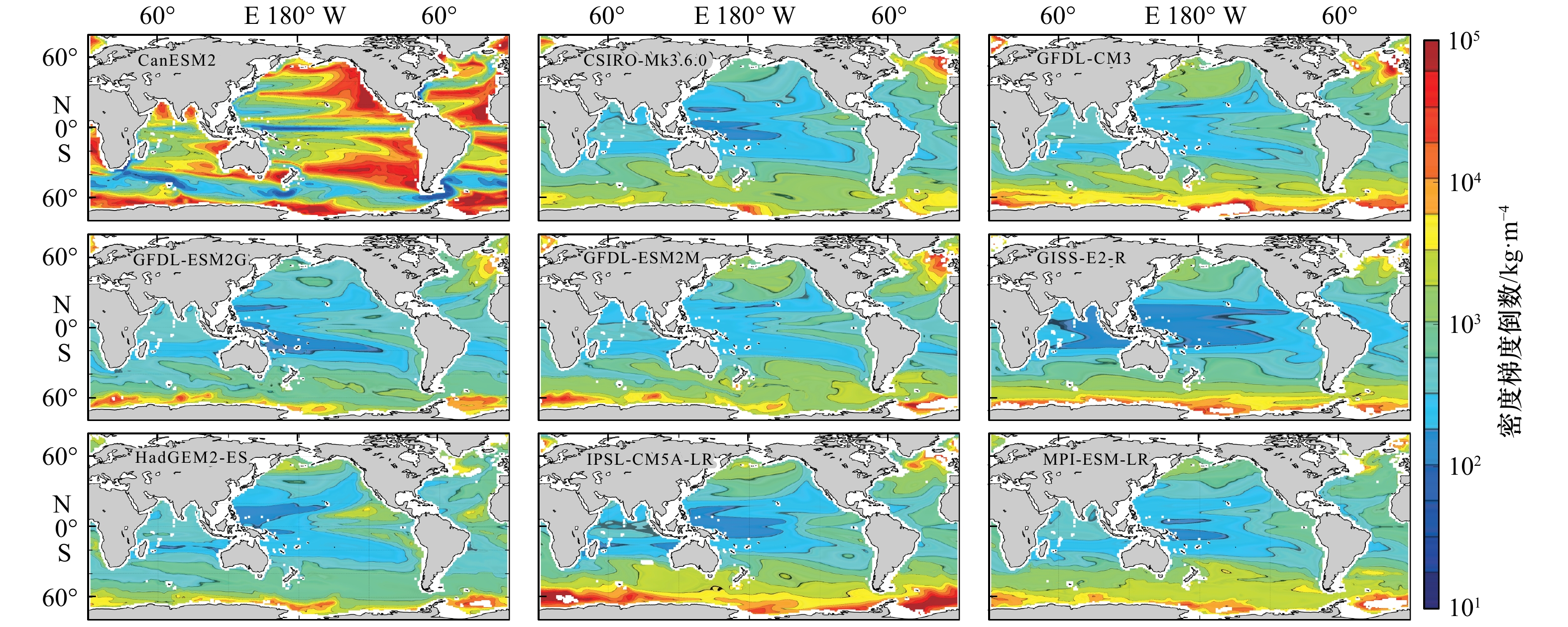
图 8 各模式密度梯度倒数项的空间分布
Fig. 8 Spatial distribution of the reciprocal of density gradient in each model

图 9 中尺度有效重力势能(EAGPE)、扰动密度平方以及密度梯度倒数的空间分布
a−c为Argo观测计算结果,d−f为多模式集合平均计算结果,g−i为Argo观测结果与多模式集合平均的偏差
Fig. 9 Spatial distribution of EAGPE, the square of density perturbation and the reciprocal of density gradient
a−c are the results from Argo observation, d−f are the results from assemble average of multi-models, and g−i are the difference between Argo observation and the assemble average of multi-models
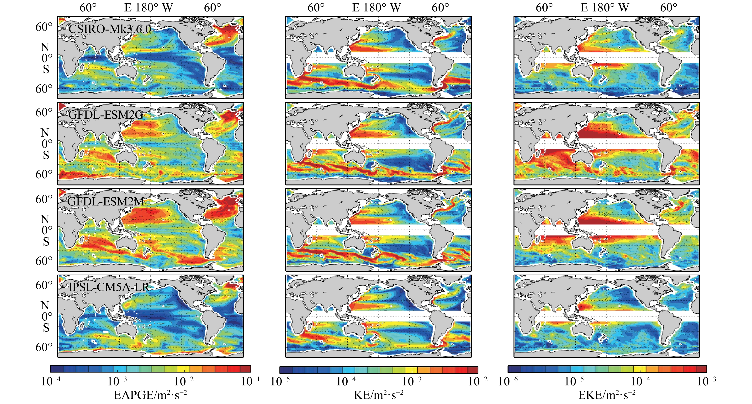
图 10 由模式计算的中尺度有效重力势能(EAGPE)、动能(KE)、涡动能(EKE)的空间分布
Fig. 10 Spatial distribution of EAGPE, KE and EKE calculated from model outputs
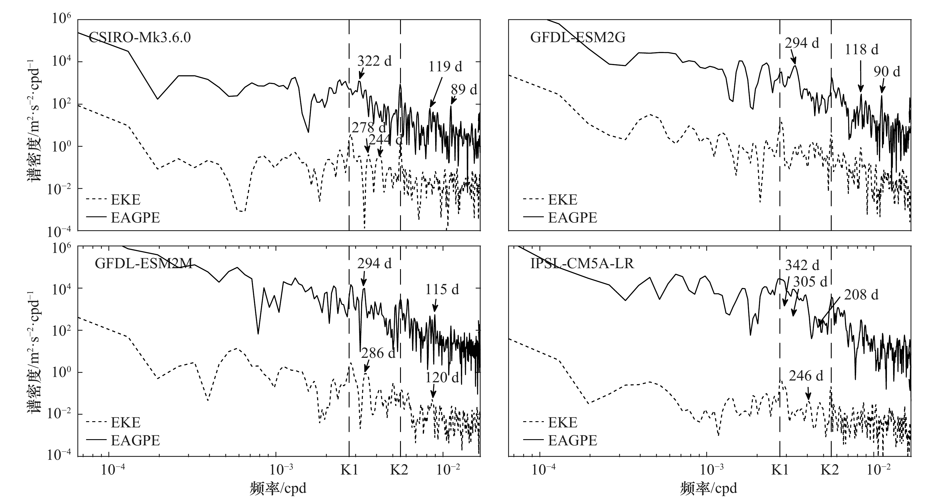
图 11 黑潮区域涡动能(EKE)与中尺度有效重力势能(EAGPE)时间序列的功率谱
Fig. 11 Power spectral of EKE and EAGPE in the Kuroshio region
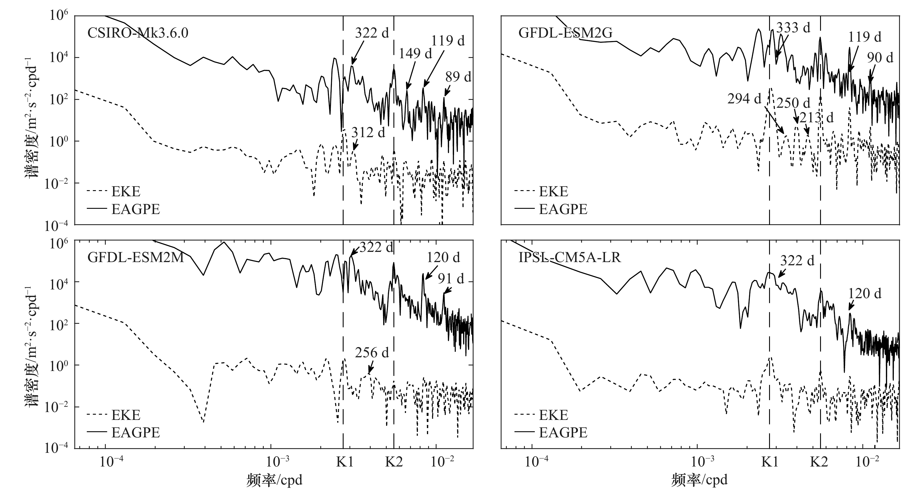
图 12 北大西洋湾流区域涡动能(EKE)与中尺度有效重力势能(EAGPE)时间序列的功率谱
Fig. 12 Power spectral of EKE and EAGPE in the gulf stream region of North Atlantic
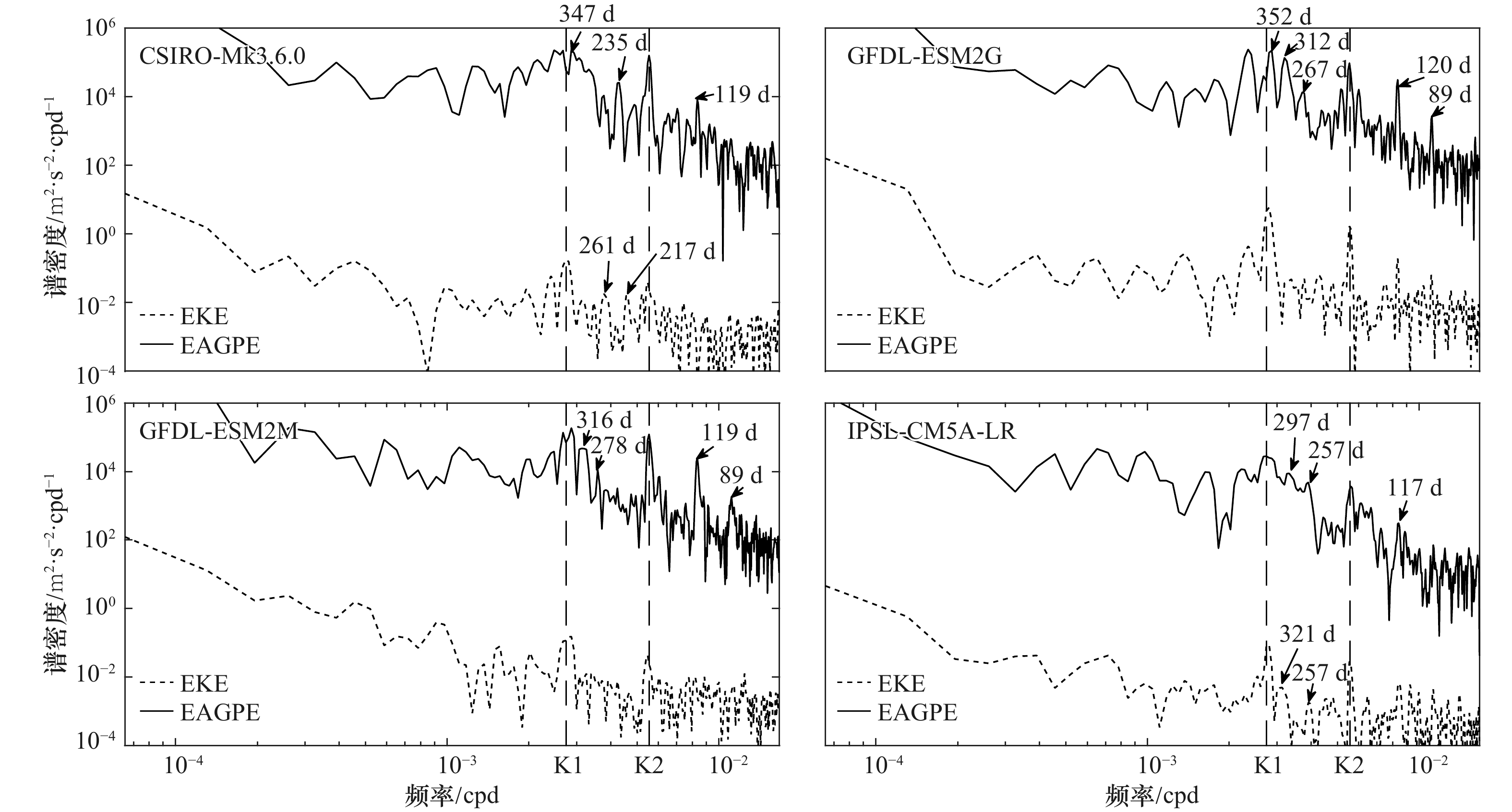
图 13 南大洋区域涡动能(EKE)与中尺度有效重力势能(EAGPE)时间序列功率谱
Fig. 13 Power spectral of EKE and EAGPE in the Southern Ocean region
表 1 模式介绍
Tab. 1 Models introduction
模式 网格 垂向混合方案 参考 CanESM2 256×192 KPP+TM Chylek等[26] CSIRO-Mk3.6.0 192×189 KT BML Gordon等[27] GFDL-CM3 360×200 KPP+TM Griffies等[28] GFDL-ESM2G 360×210 BML[29]+SME+TM Dunne等[30] GFDL-ESM2M 360×200 KPP+SME+TM Dunne等[30] GISS-E2-R 288×180 KPP Liu等[31] HadGEM2-ES 360×216 KT BML+内部参数化调整[32] Martin[33],Johns等[34] IPSL-CM5A-LR 182×149 TC[35] Dufresne等[36] MPI-ESM-LR 256×200 PP+混合层内与风速相关的参数化 Jungclaus等[37] 注:KPP:K剖面参数化方案(K-profile parameterization scheme)[38];KT:Kraus和Turner[39]方案;BML:整体混合层方案(bulk mixed layer scheme);SME:中尺度涡对混合层再分层的参数化(parameterization of mixed layer restratification by submesoscale eddies)[40];TM:潮汐驱动混合参数化方案(tidally driven mixing parameterization);TC:湍流闭合方案(turbulence closure scheme);PP:Pacanowski和Philander方案[41]。  下载: 导出CSV
表 2 涡动能(EKE)与中尺度有效重力势能(EAGPE)时间序列相关性
Tab. 2 The correlation between the temporal variations of EKE and EAGPE
区域 CSIRO-Mk3.6.0 GFDL-ESM2G GFDL-ESM2M IPSL-CM5A-LR 黑潮区域 0.397 0.462 0.438 0.181 南大洋区域 0.262 0.308 0.557 0.147 北大西洋湾流 0.097 0.145 −0.323 0.144
下载: 导出CSV
-
[1] Taylor K E, Stouffer R J, Meehl G A. An overview of CMIP5 and the experiment design[J]. Bulletin of the American Meteorological Society, 2012, 93(4): 485−498. doi: 10.1175/BAMS-D-11-00094.1 [2] Moss R H, Edmonds J A, Hibbard K A, et al. The next generation of scenarios for climate change research and assessment[J]. Nature, 2010, 463(7282): 747−756. doi: 10.1038/nature08823 [3] Allen S K, Plattner G K, Nauels A, et al. Climate Change 2013: The Physical Science Basis. An Overview of the Working Group 1 Contribution to the Fifth Assessment Report of the Intergovernmental Panel on Climate Change (IPCC)[C]. Vienna, Austria: AGU, 2013. [4] Smith T M, Reynolds R W. Improved extended reconstruction of SST (1854–1997)[J]. Journal of Climate, 2004, 17(12): 2466−2477. doi: 10.1175/1520-0442(2004)017<2466:IEROS>2.0.CO;2 [5] Compo G P, Whitaker J S, Sardeshmukh P D, et al. The twentieth century reanalysis project[J]. Quarterly Journal of the Royal Meteorological Society, 2011, 137(654): 1−28. doi: 10.1002/qj.776 [6] Carton J A, Giese B S. A reanalysis of ocean climate using Simple Ocean Data Assimilation (SODA)[J]. Monthly Weather Review, 2008, 136(8): 2999−3017. doi: 10.1175/2007MWR1978.1 [7] Wang C Z, Zhang L P, Lee S K, et al. A global perspective on CMIP5 climate model biases[J]. Nature Climate Change, 2014, 4(3): 201−205. doi: 10.1038/nclimate2118 [8] Huang C J, Qiao F L, Dai D J. Evaluating CMIP5 simulations of mixed layer depth during summer[J]. Journal of Geophysical Research: Oceans, 2014, 119(4): 2568−2582. doi: 10.1002/2013JC009535 [9] Oort A H, Anderson L A, Peixoto J P. Estimates of the energy cycle of the oceans[J]. Journal of Geophysical Research: Oceans, 1994, 99(C4): 7665−7688. doi: 10.1029/93JC03556 [10] 冯洋. 大洋有效位能及浮力通量对其作用机制研究[D]. 青岛: 中国海洋大学, 2006.Feng Yang. The available potential energy in the world oceans and its sources/sinks from surface buoyancy flux[D]. Qingdao: Ocean University of China, 2006. [11] Chen R, McClean J L, Gille S T, et al. Isopycnal eddy diffusivities and critical layers in the Kuroshio Extension from an eddying ocean model[J]. Journal of Physical Oceanography, 2014, 44(8): 2191−2211. doi: 10.1175/JPO-D-13-0258.1 [12] Bray N A, Fofonoff N P. Available potential energy for MODE eddies[J]. Journal of Physical Oceanography, 1981, 11(1): 30−47. doi: 10.1175/1520-0485(1981)011<0030:APEFME>2.0.CO;2 [13] Sandström J W, Helland-Hansen B. über die Berechnung von Meeresströmungen[J]. Norwegion Fisheries Invest, 1903, 2(4): 43. [14] Huang R X. Mixing and available potential energy in a Boussinesq ocean[J]. Journal of Physical Oceanography, 1998, 28(4): 669−678. doi: 10.1175/1520-0485(1998)028<0669:MAAPEI>2.0.CO;2 [15] Oort A H, Ascher S C, Levitus S, et al. New estimates of the available potential energy in the world ocean[J]. Journal of Geophysical Research: Oceans, 1989, 94(C3): 3187−3200. doi: 10.1029/JC094iC03p03187 [16] Pedlosky J. Geophysical Fluid Dynamics[M]. New York: Springer Science & Business Media, 1979. [17] Wright W R. Northern sources of energy for the deep Atlantic[J]. Deep Sea Research and Oceanographic Abstracts, 1972, 19(12): 865−877. doi: 10.1016/0011-7471(72)90004-6 [18] Lorenz E N. Available potential energy and the maintenance of the general circulation[J]. Tellus, 1955, 7(2): 157−167. doi: 10.3402/tellusa.v7i2.8796 [19] Nycander J. Horizontal convection with a non-linear equation of state: generalization of a theorem of Paparella and Young[J]. Tellus A: Dynamic Meteorology and Oceanography, 2010, 62(2): 134−137. doi: 10.1111/j.1600-0870.2009.00429.x [20] Tailleux R. Available potential energy and exergy in stratified fluids[J]. Annual Review of Fluid Mechanics, 2013, 45(1): 35−58. doi: 10.1146/annurev-fluid-011212-140620 [21] Winters K B, Lombard P N, Riley J J, et al. Available potential energy and mixing in density-stratified fluids[J]. Journal of Fluid Mechanics, 1995, 289: 115−128. doi: 10.1017/S002211209500125X [22] Huang R X. Available potential energy in the world's oceans[J]. Journal of Marine Research, 2005, 63(1): 141−158. doi: 10.1357/0022240053693770 [23] Tseng Y H, Ferziger J H. Mixing and available potential energy in stratified flows[J]. Physics of Fluids, 2001, 13(5): 1281−1293. doi: 10.1063/1.1358307 [24] Saenz J A, Tailleux R, Butler E D, et al. Estimating Lorenz’s reference state in an ocean with a nonlinear equation of state for seawater[J]. Journal of Physical Oceanography, 2015, 45(5): 1242−1257. doi: 10.1175/JPO-D-14-0105.1 [25] Feng Y, Wang W, Huang R X. Meso-scale available gravitational potential energy in the world oceans[J]. Acta Oceanologica Sinica, 2006, 25(5): 1−13. [26] Chylek P, Li J, Dubey M K, et al. Observed and model simulated 20th century Arctic temperature variability: Canadian earth system model CanESM2[J]. Atmospheric Chemistry and Physics Discussions, 2011, 11(8): 22893−22907. doi: 10.5194/acpd-11-22893-2011 [27] Gordon H, O'Farrell S, Collier M, et al. The CSIRO Mk3.5 climate model[R]. Aspendale, Victoria, Australia: The Center for Australian Weather and Climate Research, 2010: 62. [28] Griffies S M, Winton M, Donner L J, et al. The GFDL CM3 coupled climate model: characteristics of the ocean and sea ice simulations[J]. Journal of Climate, 2011, 24(13): 3520−3544. doi: 10.1175/2011JCLI3964.1 [29] Hallberg R. The ability of large-scale ocean models to accept parameterizations of boundary mixing, and a description of a refined bulk mixed-layer model[C]//Proceedings of the 2003‘Aha Huliko’a Hawaiian Winter Workshop. Honolulu, HI: University of Hawaii, 2003: 187-203. [30] Dunne J P, John J G, Adcroft A J, et al. GFDL’s ESM2 global coupled climate-carbon earth system models. Part I: Physical formulation and baseline simulation characteristics[J]. Journal of Climate, 2012, 25(19): 6646−6665. doi: 10.1175/JCLI-D-11-00560.1 [31] Liu J P, Schmidt G A, Martinson D G, et al. Sensitivity of sea ice to physical parameterizations in the GISS global climate model[J]. Journal of Geophysical Research: Oceans, 2003, 108(C2): 3053. [32] Peters H, Gregg M C, Toole J M. On the parameterization of equatorial turbulence[J]. Journal of Geophysical Research: Oceans, 1988, 93(C2): 1199−1218. doi: 10.1029/JC093iC02p01199 [33] Martin P J. Simulation of the mixed layer at OWS November and Papa with several models[J]. Journal of Geophysical Research: Oceans, 1985, 90(C1): 903−916. doi: 10.1029/JC090iC01p00903 [34] Johns T C, Durman C F, Banks H T, et al. The new Hadley Centre climate model (HadGEM1): evaluation of coupled simulations[J]. Journal of Climate, 2006, 19(7): 1327−1353. doi: 10.1175/JCLI3712.1 [35] Madec G, Pascale Delécluse, Imbard M, et al. OPA 8.1 ocean general circulation model reference manual[S]. Note Du Pole De Modélisation Institut Pierre Simon Laplace, 2007: 11. [36] Dufresne J L, Foujols M A, Denvil S, et al. Climate change projections using the IPSL-CM5 Earth System Model: from CMIP3 to CMIP5[J]. Climate Dynamics, 2013, 40(9/10): 2123−2165. [37] Jungclaus J H, Fischer N, Haak H, et al. Characteristics of the ocean simulations in the Max Planck Institute Ocean Model (MPIOM) the ocean component of the MPI-earth system model[J]. Journal of Advances in Modeling Earth Systems, 2013, 5(2): 422−446. doi: 10.1002/jame.20023 [38] Large W G, McWilliams J C, Doney S C. Oceanic vertical mixing: a review and a model with a nonlocal boundary layer parameterization[J]. Reviews of Geophysics, 1994, 32(4): 363−403. doi: 10.1029/94RG01872 [39] Kraus E B, Turner J S. A one-dimensional model of the seasonal thermocline II. The general theory and its consequences[J]. Tellus, 1967, 19(1): 98−106. doi: 10.3402/tellusa.v19i1.9753 [40] Fox-Kemper B, Danabasoglu G, Ferrari R, et al. Parameterization of mixed layer eddies. III: Implementation and impact in global ocean climate simulations[J]. Ocean Modelling, 2011, 39(1/2): 61−78. [41] Pacanowski R C, Philander S G H. Parameterization of vertical mixing in numerical models of tropical oceans[J]. Journal of Physical Oceanography, 1981, 11(11): 1443−1451. [42] Wiin-Nielsen A, Chen T C. Fundamentals of Atmospheric Energetics[M]. Oxford: Oxford University Press, 1993. [43] Dutton J A, Johnson D R. The theory of available potential energy and a variational approach to atmospheric energetics[J]. Advances in Geophysics, 1967, 12: 333−436. doi: 10.1016/S0065-2687(08)60379-9 [44] Kang D J, Fringer O. On the calculation of available potential energy in internal wave fields[J]. Journal of Physical Oceanography, 2010, 40(11): 2539−2545. doi: 10.1175/2010JPO4497.1 [45] Venayagamoorthy S K. Nonhydrostatic and nonlinear contributions to the energy flux budget in nonlinear internal waves[J]. Geophysical Research Letters, 2005, 32(15): L15603. doi: 10.1029/2005GL023432 [46] Moum J N, Klymak J M, Nash J D, et al. Energy transport by nonlinear internal waves[J]. Journal of Physical Oceanography, 2007, 37(7): 1968−1988. doi: 10.1175/JPO3094.1 [47] Klymak J M, Moum J N. Internal solitary waves of elevation advancing on a shoaling shelf[J]. Geophysical Research Letters, 2003, 30(20): 2045. [48] Klymak J M, Pinkel R, Liu C T, et al. Prototypical solitons in the South China Sea[J]. Geophysical Research Letters, 2006, 33(11): L11607. doi: 10.1029/2006GL025932 [49] Wang T, Geyer W R. The balance of salinity variance in a partially stratified estuary: implications for exchange flow, mixing, and stratification[J]. Journal of Physical Oceanography, 2018, 48(12): 2887−2899. doi: 10.1175/JPO-D-18-0032.1 [50] Osborn T R, Cox C S. Oceanic fine structure[J]. Geophysical Fluid Dynamics, 1972, 3(4): 321−345. doi: 10.1080/03091927208236085 [51] Burchard H, Rennau H. Comparative quantification of physically and numerically induced mixing in ocean models[J]. Ocean Modelling, 2008, 20(3): 293−311. doi: 10.1016/j.ocemod.2007.10.003 [52] 张宇, 林一骅, 王辉. 垂直湍流输送对大洋的重力位能和混合过程的影响[J]. 大气科学, 2014, 38(5): 838−844.Zhang Yu, Lin Yihua, Wang Hui. Impact of vertical turbulence on ocean gravitational potential energy and the tracer mixing process[J]. Chinese Journal of Atmospheric Sciences, 2014, 38(5): 838−844. -

计量
- 文章访问数: 285
- HTML全文浏览量: 86
- PDF下载量: 33
- 被引次数: 0
