基于非线性薛定谔方程的波浪预报方法研究

张新宇; 韩佳; 王骁; 石爱国

doi:10.3969/j.issn.0253-4193.2019.11.002

基于非线性薛定谔方程的波浪预报方法研究

doi: 10.3969/j.issn.0253-4193.2019.11.002

张新宇^1,,
韩佳²,
王骁^1, ,,
石爱国¹

1.
大连舰艇学院航海系，辽宁大连 116018
2.
解放军31010部队，北京 100081

详细信息

作者简介:
张新宇（1989—），男，山东省高密市人，博士，从事海浪预报相关研究。E-mail：zhang-xy08@163.com

通讯作者:
王骁（1980—），男，辽宁省沈阳市人，博士，从事海浪预报及船舶摇荡预报相关研究。E-mail：1748692208@qq.com

中图分类号: P733
计量
- 文章访问数: 390
- HTML全文浏览量: 26
- PDF下载量: 112
- 被引次数: 0
出版历程
- 收稿日期: 2018-08-19
- 修回日期: 2019-02-02
- 网络出版日期: 2021-04-21
- 刊出日期: 2019-11-25

Research on wave prediction method based on nonlinear Schrödinger equation

Zhang Xinyu^1
,,
Han Jia²,
Wang Xiao^{1
, ,},
Shi Aiguo¹

1.
Dalian Naval Academy, Dalian 116018, China
2.
PLA Unit of 31010, Beijing 100081, China

摘要

摘要: 为探索海浪波面信息的实时预报方法，以三阶非线性薛定谔(NLS)方程的逆散射变换求解为基础，通过理论推导，给出了一种由实测波高时历数据计算其NLS方程本征值的方法，进一步实现了对波浪包络时空演变的预报。通过预报结果与实测波列的比对，验证了方法的有效性和准确性。该方法可为船舶或海上平台的大浪预警，以及为大波浪中海上作业寻找窗口期等提供一条新的技术途径。
- NLS方程 /
- 逆散射变换 /
- 本征值 /
- 预报
Abstract: In order to study the real-time prediction method of ocean wave information, some theoretical derivation is made based on inverse scattering transformation of cubic Schrödinger equation, and a method to calculate eigenvalues from measured wave height time series is given. Then the calculated eigenvalues are used to predict spatial-temporal evolution of wave envelope. The predictions are then compared with measured time series, the results show the method has good effectiveness and accuracy. This method can provide support for big wave warning of ships or offshore platform, and time windows seeking for offshore operation under heavy sea.
- nonlinear Schrödinger equation /
- inverse scattering transform /
- eigenvalues /
- predict

HTML全文

图 1 黎曼θ函数解图像

Fig. 1 Figure of a Riemann θ function solution

下载: 全尺寸图片幻灯片

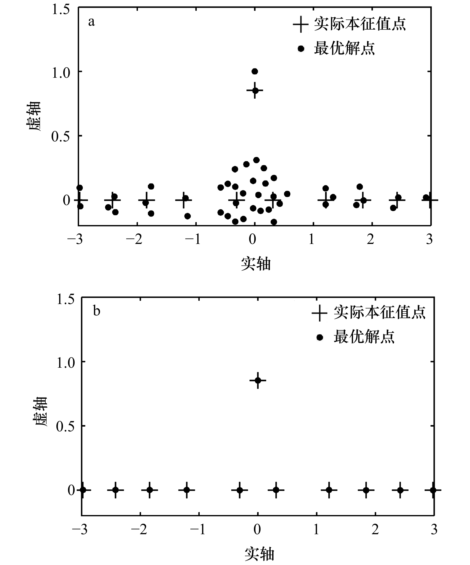
图 2 $A = 1,\;T = 6$ s时寻优效果示意图

a. 10次迭代后优化结果；b. 最终寻优结果

Fig. 2 Figure of optimization when $A = 1$ and $T = 6$ s

a. Optimization result after 10 steps of iteration; b. the final optimization result

下载: 全尺寸图片幻灯片

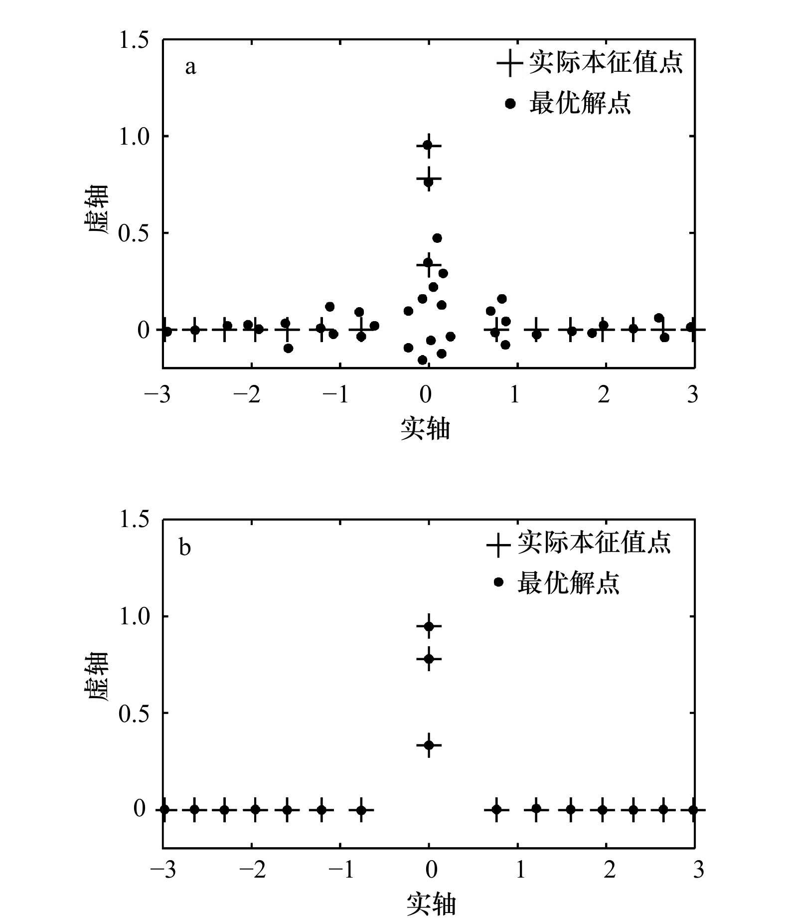
图 3 $A = 1,\;T = 10$ s时寻优效果示意图

a. 10次迭代后优化结果；b. 最终寻优结果

Fig. 3 Figure of optimization when $A = 1$ and $T = 10$ s

a. Optimization result after 10 steps of iteration; b. the final optimization result

下载: 全尺寸图片幻灯片

图 4 $x = 0$处的波包络时间序列

Fig. 4 Wave envelope time series at the point $x = 0$

下载: 全尺寸图片幻灯片

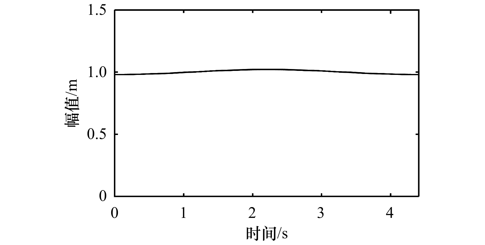
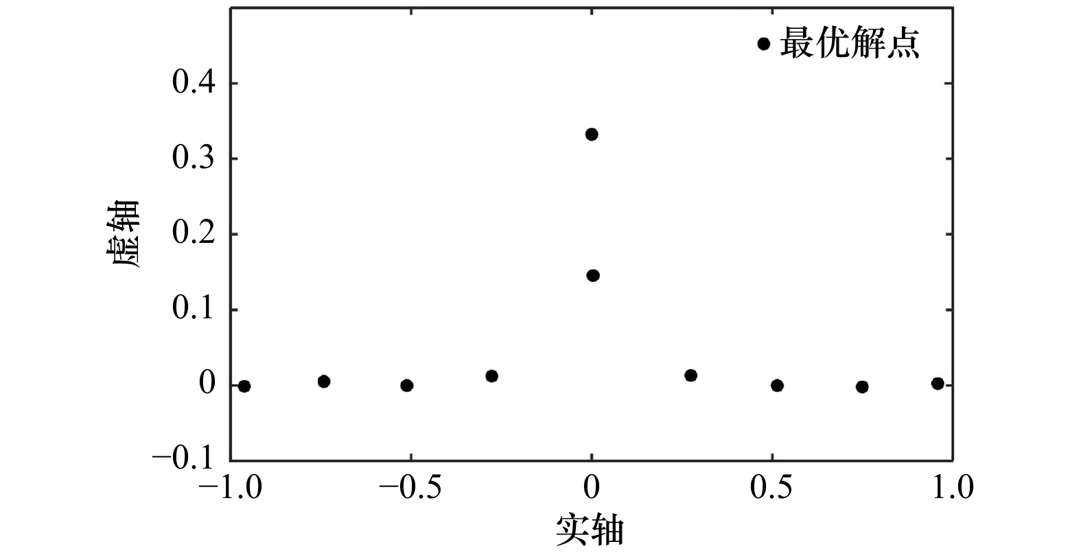
图 5 $x = 0$处序列的优化结果

Fig. 5 The final optimization result of the series at the point $x = 0$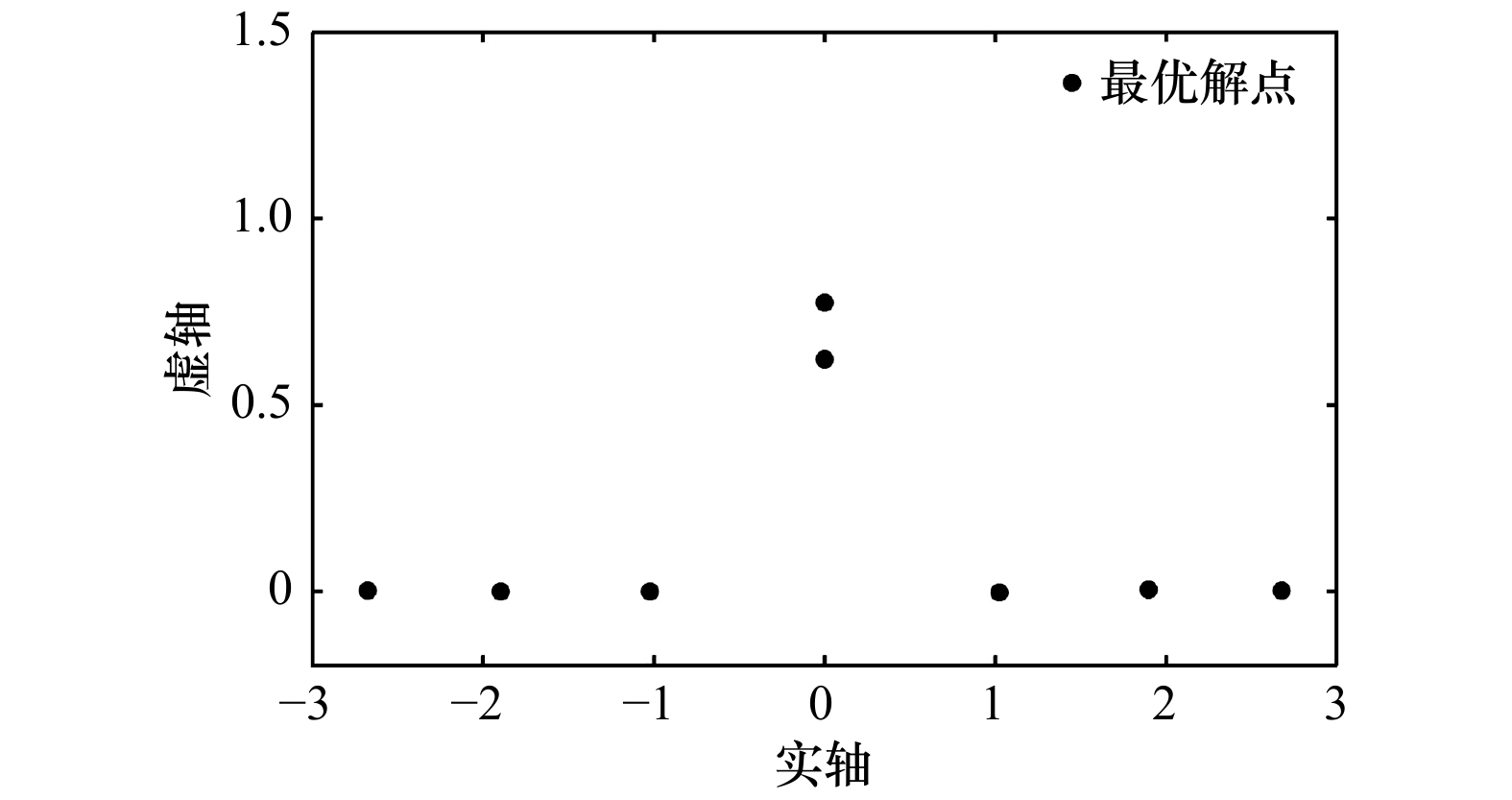

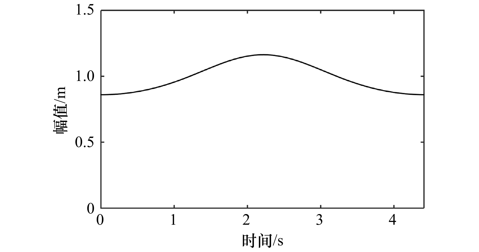
下载: 全尺寸图片幻灯片

图 6 $x = 1$处的波包络时间序列

Fig. 6 Wave envelope time series at the point $x = 1$

下载: 全尺寸图片幻灯片

图 7 $x = 1$处序列的优化结果

Fig. 7 The final optimization result of the series at the point $x = 1$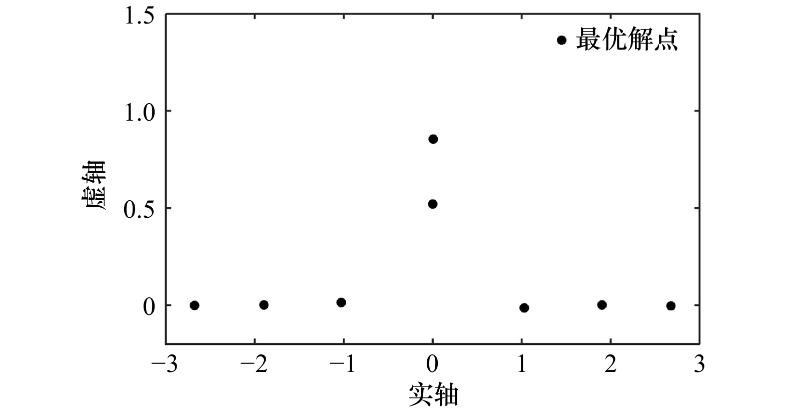

下载: 全尺寸图片幻灯片

图 8 $x = 1.5$处的波包络时间序列

Fig. 8 Wave envelope time series at the point $x = 1.5$

下载: 全尺寸图片幻灯片

图 9 $x = 1.5$处序列的优化结果

Fig. 9 The final optimization result of the series at the point $x = 1.5$

下载: 全尺寸图片幻灯片

图 10 台南水力学实验室水池实验数据

Fig. 10 Experiment data of Tainan Hydraulics Laboratory

下载: 全尺寸图片幻灯片

图 11 单周期波列数据

Fig. 11 Wave data of single period

下载: 全尺寸图片幻灯片

图 12 初始波列及其包络

Fig. 12 The initial wave train and its envelope

下载: 全尺寸图片幻灯片

图 13 初始波列及其包络

Fig. 13 The initial wave train and its envelope

下载: 全尺寸图片幻灯片

图 14 黎曼θ函数解图像

Fig. 14 Figure of a Riemann θ function solution

下载: 全尺寸图片幻灯片

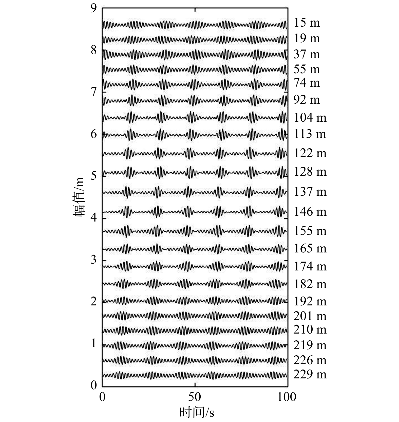
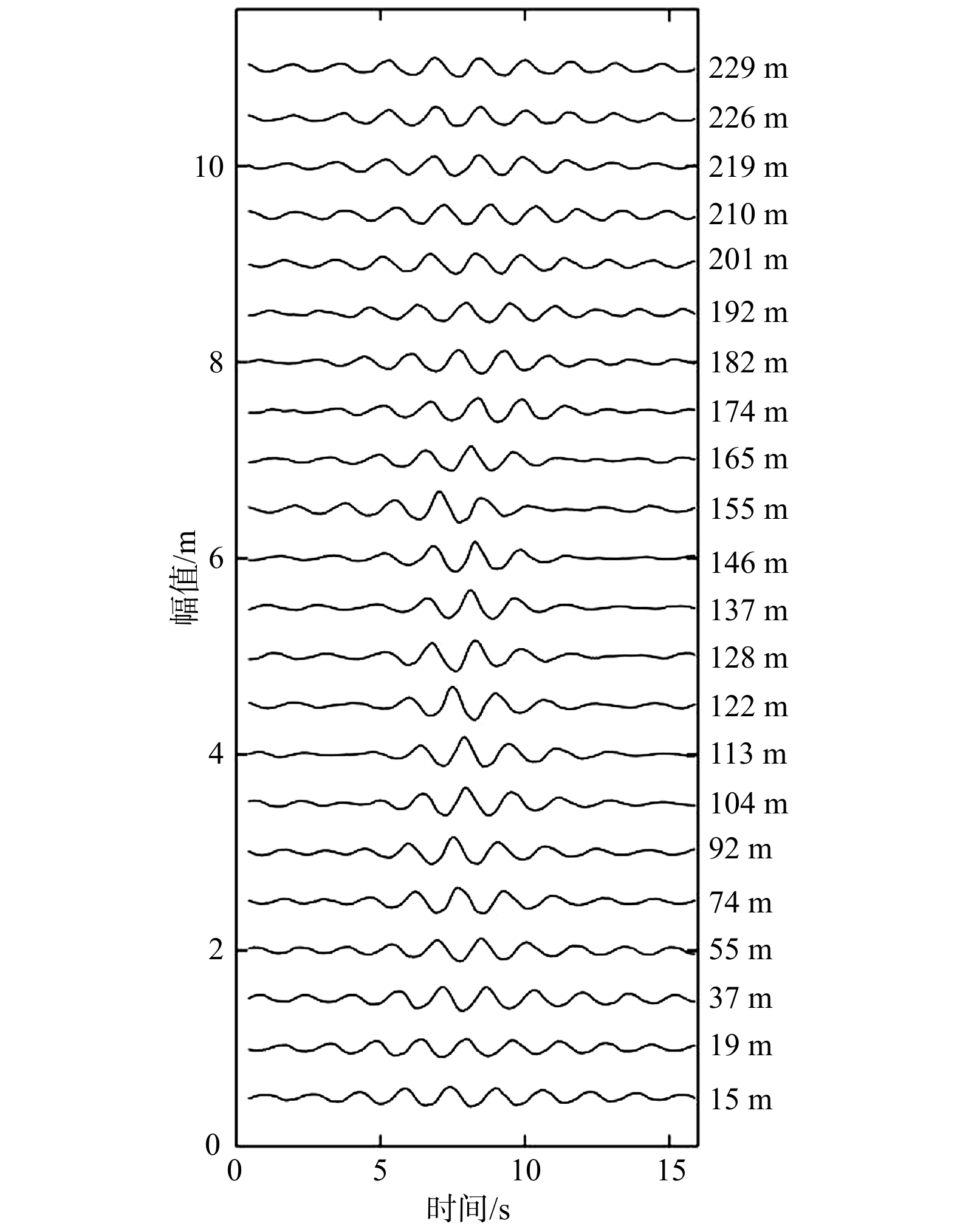
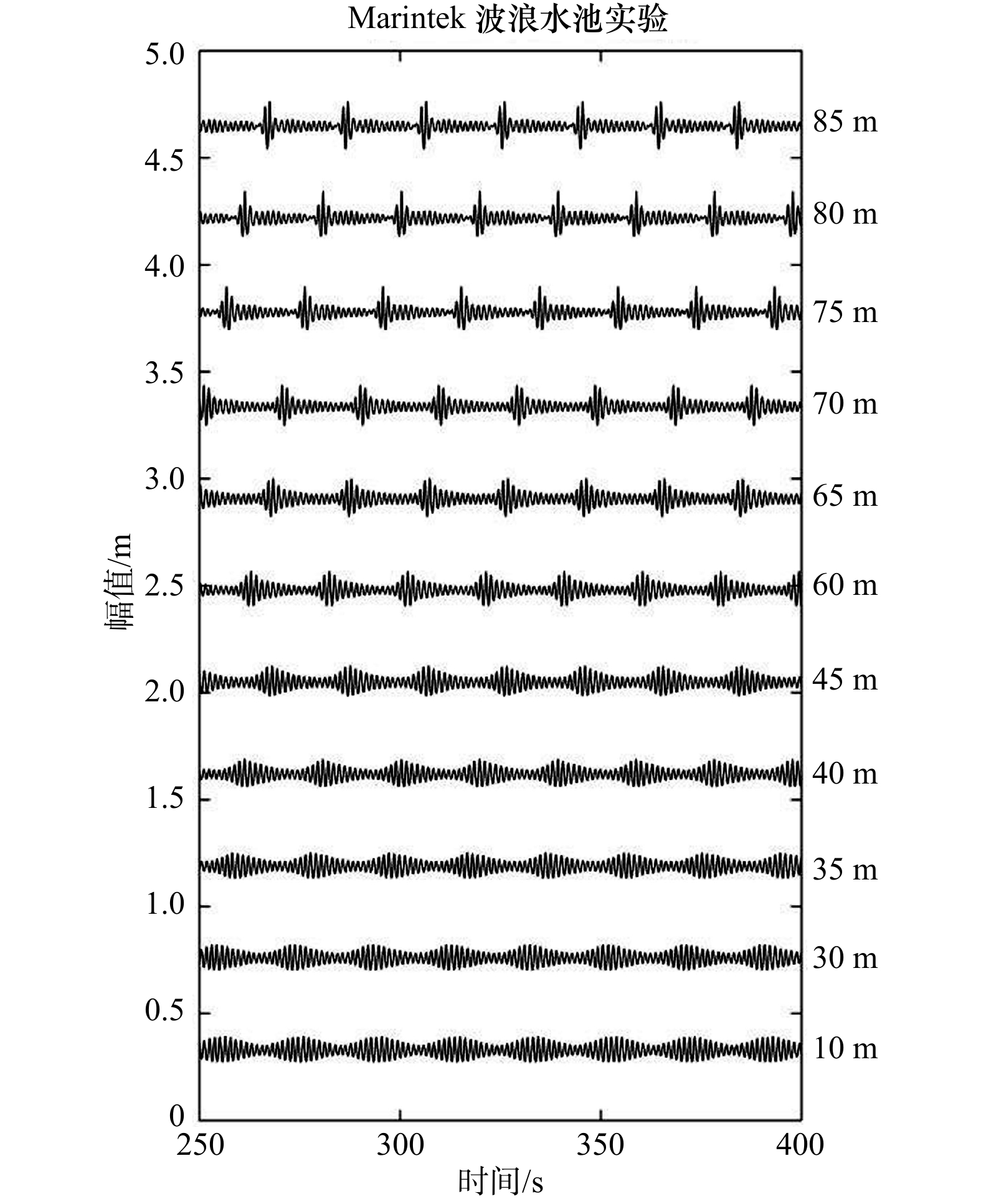
图 15 第3个波高传感器（37 m）处实测波列与预报包络

Fig. 15 The measured wave train and predicted envelope at the third probe (37 m)

下载: 全尺寸图片幻灯片

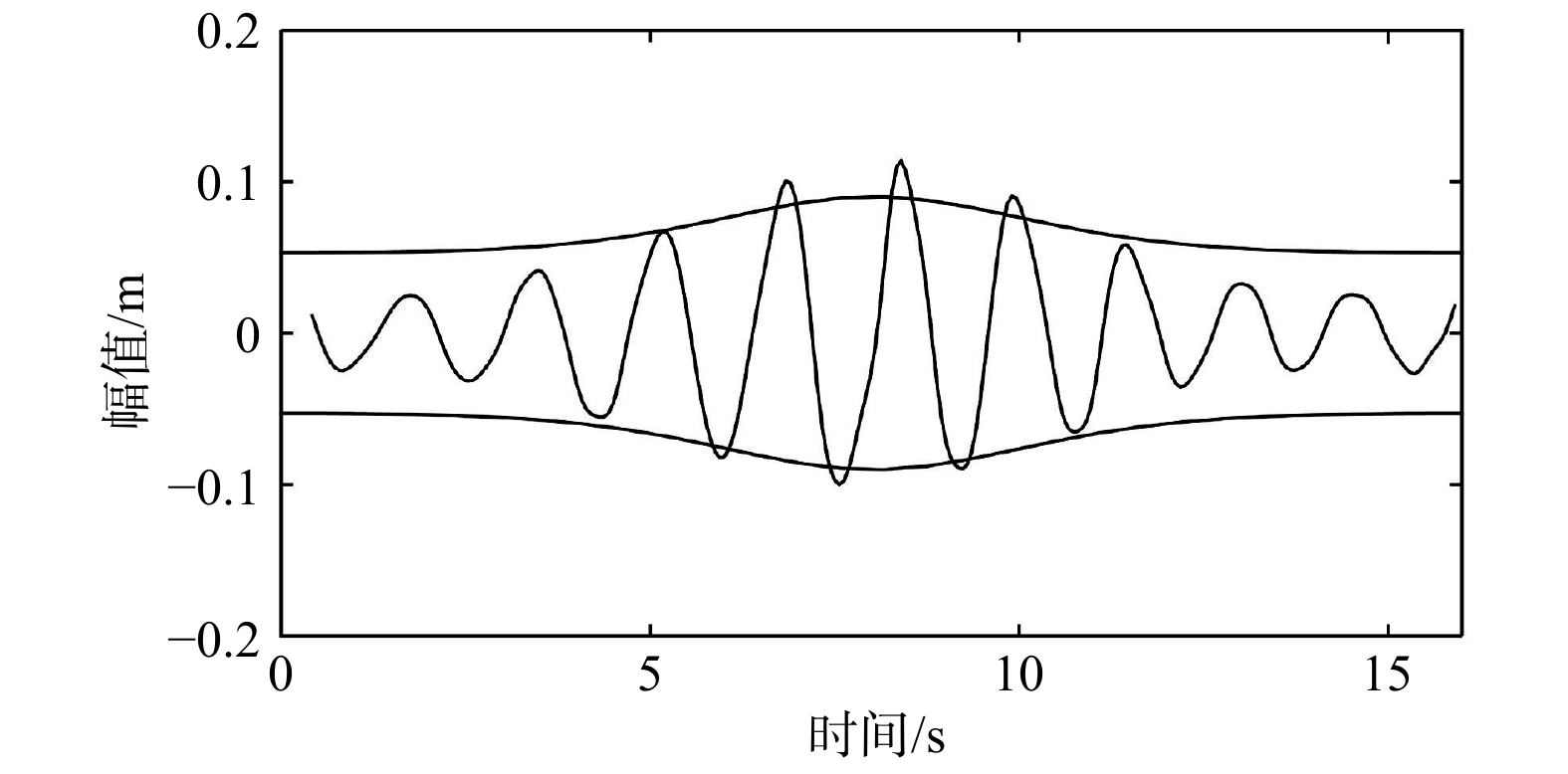
图 19 第22个波高传感器（229 m）处实测波列与预报包络

Fig. 19 The measured wave train and predicted envelope at the twenty-second probe (229 m)

下载: 全尺寸图片幻灯片

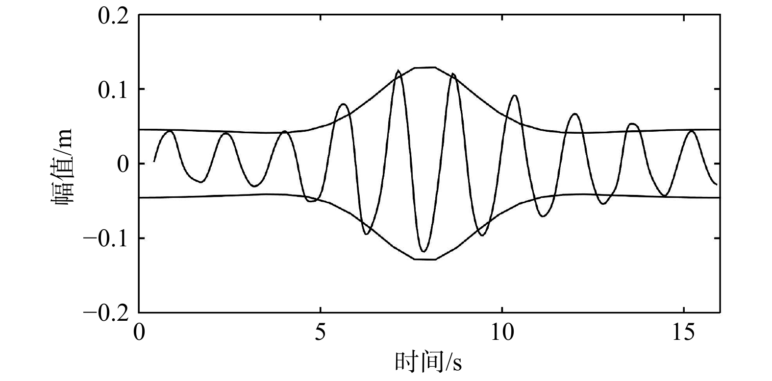
图 16 第5个波高传感器（74 m）处实测波列与预报包络

Fig. 16 The measured wave train and predicted envelope at the fifth probe (74 m)

下载: 全尺寸图片幻灯片

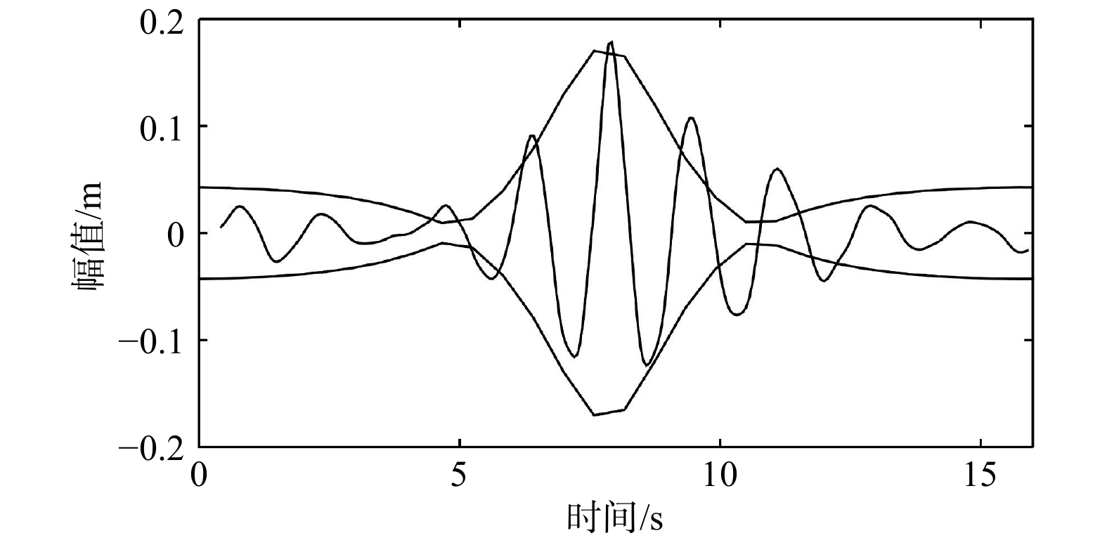
图 17 第10个波高传感器（128 m）处实测波列与预报包络

Fig. 17 The measured wave train and predicted envelope at the tenth probe (128 m)

下载: 全尺寸图片幻灯片

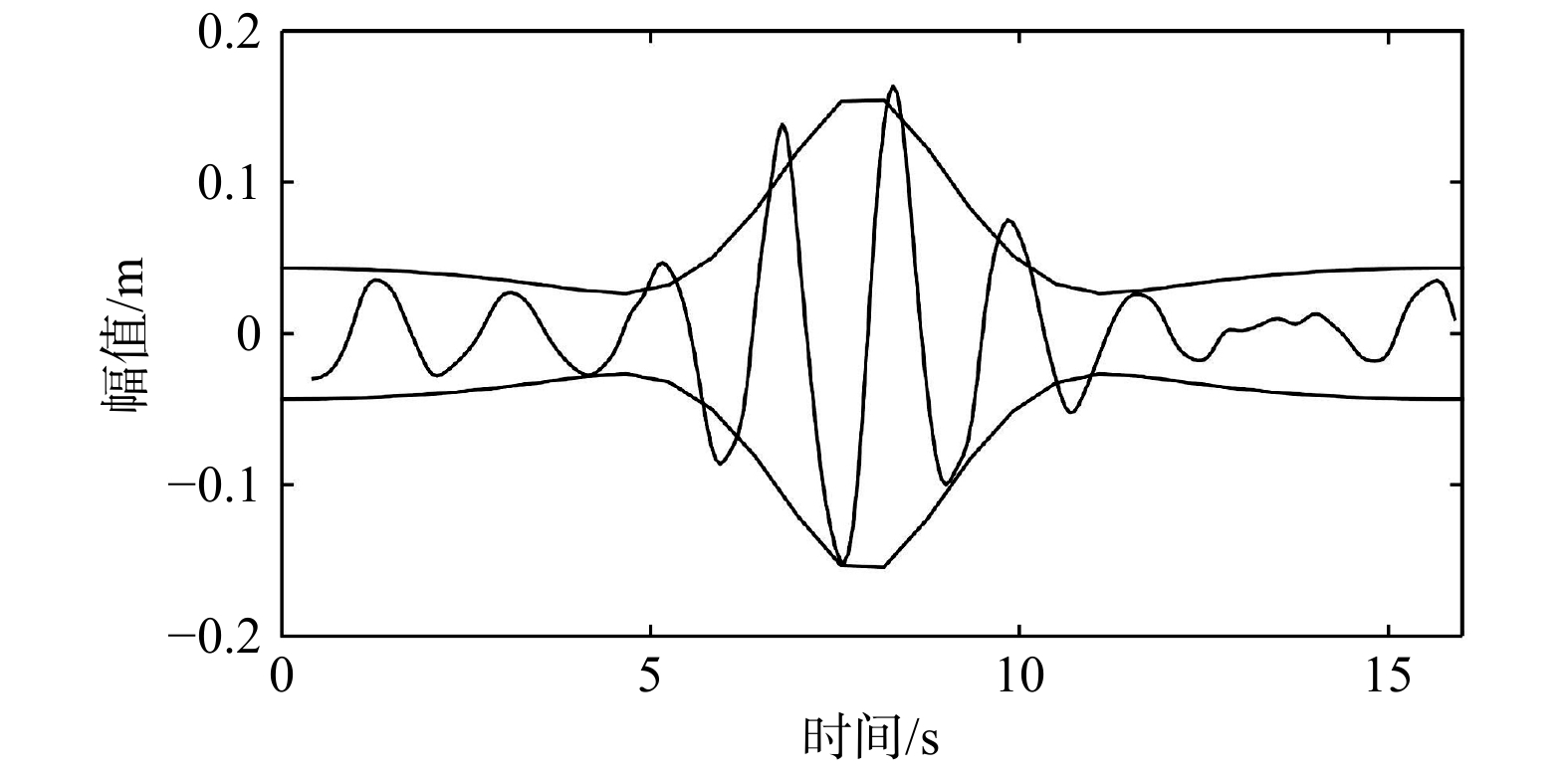
图 18 第12个波高传感器（146 m）处实测波列与预报包络

Fig. 18 The measured wave train and predicted envelope at the twelfth probe (146 m)

下载: 全尺寸图片幻灯片

图 20 Marintek水池实验结果

Fig. 20 Experiment data at Marintek

下载: 全尺寸图片幻灯片

图 21 黎曼θ函数解图像

Fig. 21 Figure of a Riemann θ function solution

下载: 全尺寸图片幻灯片

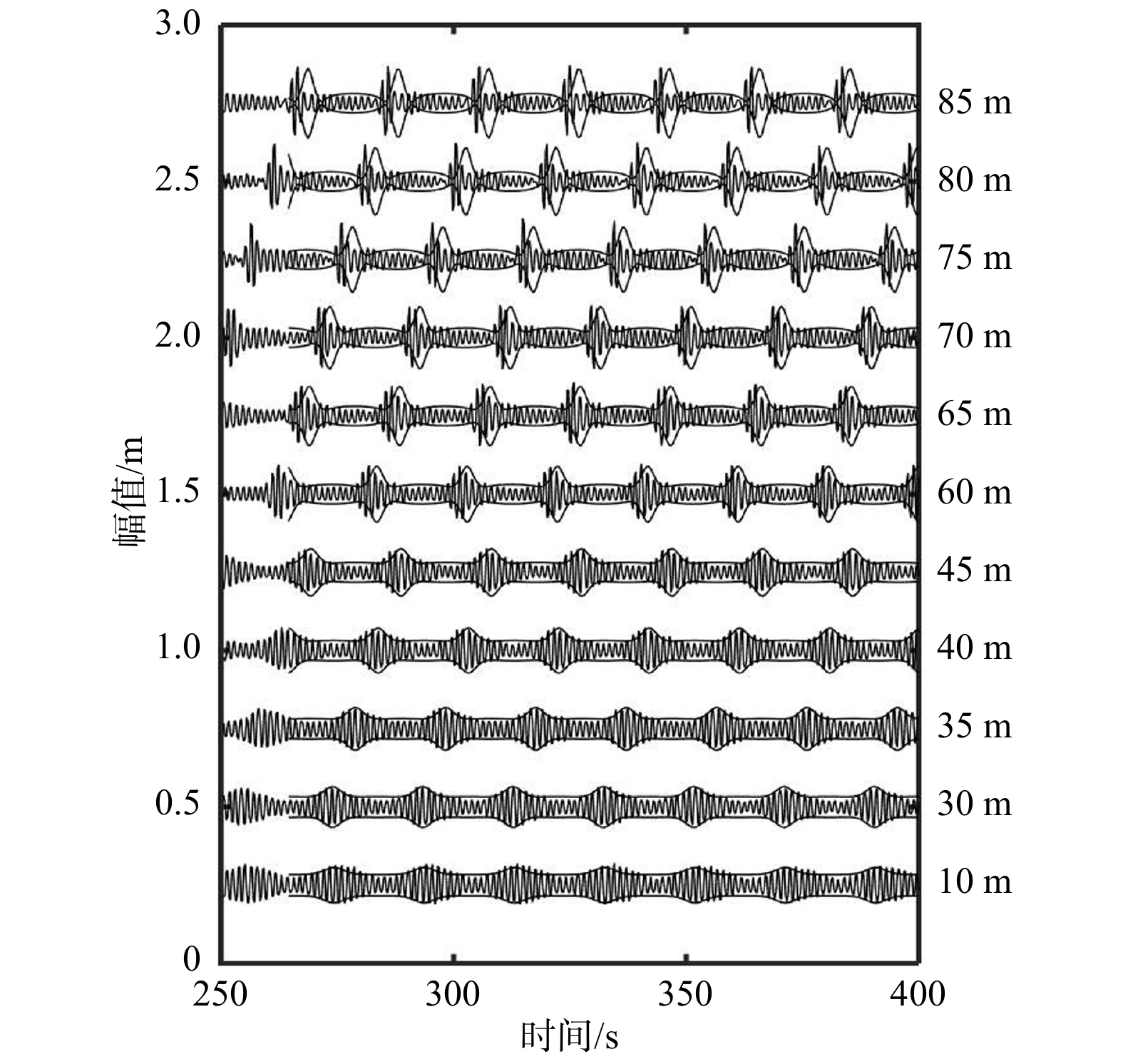
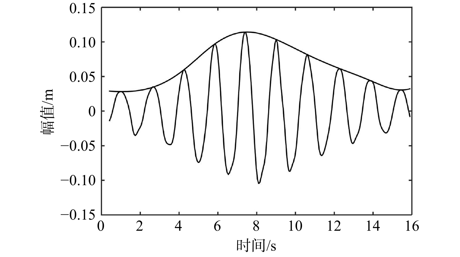
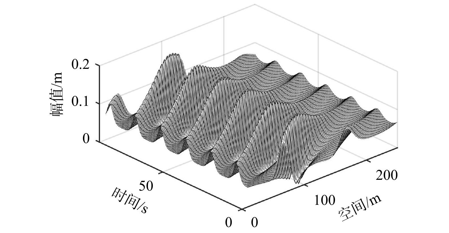
图 22 实测波列与预报包络对比

Fig. 22 Comparation between measured wave train and predicted envelope

下载: 全尺寸图片幻灯片

图 23 平移后实测波列与预报包络对比

Fig. 23 Comparation between measured wave train and predicted envelope after translation

下载: 全尺寸图片幻灯片

表 1 $A = 1,\;T = 10$ s时实际本征值与仿真结果对比

Tab. 1 Comparison of real eigenvalues and simulation resultwhen A=1 and T=10 s

实际本征值位置	对应寻优结果
0.000 0+0.949 4i	0.001 1+0.948 7i
0.000 0+0.778 0i	–0.000 7+0.776 9i
0.000 0+0.334 3i	–0.000 2+0.334 2i
0.761 0+0.000 0i	0.762 1+0.001 8i
–0.761 0+0.000 0i	–0.761 7–0.003 3i
1.211 4+0.000 0i	1.212 5+0.001 4i
–1.211 4+0.000 0i	–1.212 2–0.000 5i
1.597 8+0.000 0i	1.600 5+0.000 4i
–1.597 8+0.000 0i	–1.598 7–0.000 7i
1.958 6+0.000 0i	1.954 0+0.000 4i
–1.958 6+0.000 0i	–1.960 9–0.000 0i
2.305 8+0.000 0i	2.306 9+0.000 7i
–2.305 8+0.000 0i	–2.304 9–0.002 3i
2.644 7+0.000 0i	2.644 4+0.000 3i
–2.644 7+0.000 0i	–2.644 4+0.000 3i
2.978 2+0.000 0i	2.976 1+0.002 7i
–2.978 2+0.000 0i	–2.980 1–0.000 5i

下载: 导出CSV

表 2 实测和预测最大波高对比

Tab. 2 Comparison of measured max wave height and predicted result of each probe

波高传感器与造波板距离/m	实测最大波高/m	预报最大波高/m	相对误差/%
37	0.114 3	0.100 9	11.74
55	0.094 5	0.113 2	19.74
74	0.124 7	0.130 8	4.87
92	0.122 6	0.151 8	23.78
104	0.165 6	0.156 8	15.68
113	0.156 2	0.172 9	10.74
122	0.160 9	0.175 6	9.12
128	0.178 3	0.174 6	2.06
137	0.187 7	0.168 2	10.39
146	0.163 6	0.158 7	2.99
155	0.166 3	0.148 8	10.52
165	0.161 4	0.137 0	15.12
174	0.152 8	0.127 3	16.69
182	0.142 6	0.118 6	16.78
192	0.132 2	0.110 6	16.36
201	0.121 2	0.104 3	13.88
210	0.103 9	0.099 4	4.29
219	0.106 4	0.094 6	11.13
226	0.107 0	0.091 6	14.36
229	0.113 4	0.090 2	20.50

下载: 导出CSV

表 3 各波高传感器处实测波列与预测包络对比

Tab. 3 Comparison of measured wave train and predicted envelope of each probe

与造波板距离/m	实测最大波高/m	预报最大波高/m	幅值相对误差/%	时间偏差/s
30	0.065 8	0.065 5	0.48	0.55
35	0.067 7	0.068 6	1.33	0.55
40	0.074 6	0.072 1	3.25	0.68
45	0.077 0	0.076 2	1.11	0.68
60	0.097 1	0.090 6	6.71	1.25
65	0.108 1	0.096 3	10.88	1.25
70	0.104 6	0.101 4	3.10	1.49
75	0.117 6	0.106 5	9.44	1.49
80	0.128 0	0.110 5	13.69	1.49
85	0.121 6	0.112 6	7.39	1.61

下载: 导出CSV

参考文献(10)

[1]	Zakharov V E. Stability of periodic waves of finite amplitude on the surface of a deep fluid[J]. Journal of Applied Mechanics and Technical Physics, 1968, 9(2): 190−194.
[2]	Yuen H C, Lake B M. Nonlinear dynamics of deep-water gravity waves[J]. Advances in Applied Mechanics, 1982, 22: 67−229. doi: 10.1016/S0065-2156(08)70066-8
[3]	Lax P D. Integrals of nonlinear equations of evolution and solitary waves[J]. Communications on Pure and Applied Mathematics, 1968, 21(5): 467−490. doi: 10.1002/cpa.3160210503
[4]	Zakharov V E, Shabat A B. Exact theory of two-dimensional self-focusing and one-dimensional self-modulation of waves in nonlinear media[J]. Journal of Mathematical Physics, 1972, 34(7): 62−69.
[5]	Its A R, Kotlyarov V R. Explicit formulas for solutions of a nonlinear Schrödinger equation[J]. Dopovidi Akademiï Nauk Ukraïns’koï RSR: Seria A, 1976(11): 965−968, 1051.
[6]	Tracy E R, Chen H H. Nonlinear self-modulation: An exactly solvable model[J]. Physical Review A, 1988, 37(3): 815−839. doi: 10.1103/PhysRevA.37.815
[7]	Osborne A R. Nonlinear ocean wave and the inverse scattering transform[M]//Pike R, Sabatier P. Burlington: Academic Press, 2002: 271-598.
[8]	华敏, 李响. 基于近邻刺激的改进粒子群优化算法[J]. 数学的实践与认识, 2018, 48(1): 199−206. Hua Min, Li Xiang. A particle swarm optimization algorithm based on neighbor stimulate[J]. Mathematics in Practice and Theory, 2018, 48(1): 199−206.
[9]	王皓, 高立群, 欧阳海滨. 多种群随机差分粒子群优化算法及其应用[J]. 哈尔滨工程大学学报, 2017, 38(4): 652−660. Wang Hao, Gao Liqun, Ouyang Haibin. Multi-population random differential particle swarm optimization and its application[J]. Journal of Harbin Engineering University, 2017, 38(4): 652−660.
[10]	江文山. 深水区非线性波列调变之研究[D]. 台湾: 国立成功大学, 2005. Jiang Wenshan. A study of mokulation of nonlinear wave trains in deep water[D]. Taiwan: National Cheng Kung University, 2005.